The Highly Accurate Relation Between the Radius and Mass of the White Dwarf Star From Zero to Finite Temperature

Pei, Ting-Hang

doi:10.3389/fspas.2021.799210

ORIGINAL RESEARCH article

Front. Astron. Space Sci., 01 February 2022
Sec. Stellar and Solar Physics
Volume 8 - 2021 | https://doi.org/10.3389/fspas.2021.799210

The Highly Accurate Relation Between the Radius and Mass of the White Dwarf Star From Zero to Finite Temperature

Ting-Hang Pei^*

Institute of Astronomy and Astrophysics, Academia Sinica, Taipei, Taiwan

In this research, first considering the electron–electron interaction in the high-density Fermi electron gas at T = 0 K, this interaction causes the pressure 2/137 time less than the original value. However, the pressure of the Fermi electron gas should have something to do with temperature. Then, we estimate the temperature effect using statistical mechanics and find that the complicated form of the pressure p depends on temperature at the given particle number N and volume V. According to this, the central density–mass (ρ_c-M), central density–radius (ρ_c-R), and mass–radius (M-R) relations of the white dwarf star are obtained by considering the equation of state (EOS). Traditional formula gives the problematic mass–radius relation $R \propto M^{- 1 / 3}$ for the low-density white dwarf stars because it leads to R→∞ and p→0 when M→0. We correct this relation and obtain two reasonable relations in the relativistic and nonrelativistic regions. In our EOS calculations, the central density is divided into the high-, middle-, and low-density regions. All three relations are almost unchanged until 10⁸ K in the high-density region. The temperature effect mainly affects the middle- and low-density regions, and it becomes explicitly above 10⁷ K. Our calculations can explain Sloan Digital Sky Survey observations where some white dwarf stars with a radius of more than 8 × 10³ km have larger mass than the predictions by the relativistic EOS at T = 0 K. This result tells us that the temperature effect is important for the low and middle central-density white dwarf star and also useful to estimate the inner temperature of a white dwarf star.

Introduction

The white dwarf star has been investigated for many years, and it was named first in 1922 (Holberg, 2005). It usually has a very high density with mass similar to our Sun, but the volume is small like the Earth. The Chandrasekhar mass limit is the famous restriction for the upper mass of a non-rotating and uncharged white dwarf star (Chandrasekhar, 1935; Chandrasekhar, 2012). The reported largest mass seems to be the one found in 2007, which is 1.33 times as large as the solar mass M_ʘ (Kepler et al., 2007). The white dwarf star is thought to be the type of the low to medium mass stars in the final evolution stage (Schutz, 1985; Hans and Ruffini, 1994; Mould, 2002; Misner et al., 2017). The early theory to explain its mass upper limit is based on the ideally degenerate Fermi electron gas (Chandrasekhar, 1935; Kittel and Kroemer, 1980; Schutz, 1985; Huang, 1987; Greiner et al., 1995; Honerkamp, 2002; Schwabl, 2002; Chandrasekhar, 2012). The calculation adopts all electrons like free particles occupying all energy levels until Fermi energy as they are at zero temperature (Koester and Chanmugam, 1990). It is amazing that, even in the high-temperature and high-pressure situation, the ideal Fermi gas still works to explain the existence of the white dwarf star. It makes us curious to further discuss the more detailed temperature effect through statistical mechanics.

Actually, the central temperature of the Fermi electron gas in the white dwarf star might be about 10⁷–10⁸ K (Soares, 2017), the temperature effect should be further considered to get more accurate results. The problems about surface luminosity and temperature evolution of the white dwarf stars have been discussed (D’antonia and Mazzitelli, 1990). Here, we care about the central temperature more. According to statistical mechanics, we first build the pressure produced by the Fermi electron gas at given temperature T, the number of electrons N, and the total volume V. Then, we discuss the temperature effect on the electron pressure. Next, the relations between the central density ρ_c, mass M, and radius R of the white dwarf star are derived from the equation of state (EOS). Finally, on the basis of these relations, the temperature effect is discussed and the results are compared to the Sloan Digital Sky Survey (SDSS) observations. Although the temperature is maximum at the center and minimum at the surface, we still adopt the uniform temperature approximation as most research did. After all, it is more complicated to consider the temperature varying with position, and our results imply that the uniform temperature approximation may remain valuable. Furthermore, the temperature can change with time because the white dwarf stars cool down by thermal emission. However, the cooling time is much longer than the astronomical observations, and the temperature of the white dwarf star is kept constant at each calculation in our research. If we want to compare the calculation results with the astronomical observations in several decades, then to hold the initial temperature throughout each calculation is a good enough way.

The Degenerate Fermi Electron Gas for the White Dwarf Star

First, we review the calculation of the upper mass limit for the white dwarf star. It adopts the ideally degenerate Fermi electron gas and considers the relativistic kinetic energy in the calculation (Huang, 1987; Greiner et al., 1995). Because the electron has spin s $= \pm \frac{1}{2},$ each energy state permits two electrons occupied. Each electron has the rest mass m_e, and its relativistic kinetic energy E_k at momentum p is

E_{k} = m_{e} c^{2} {{[1 + {(\frac{\overset{⇀}{p}}{m_{e} c})}^{2}]}^{1 / 2} - 1}, (1)

The Fermi electron gas with the total number N and total volume V has total kinetic energy

E_{0} = 2 m_{e} c^{2} \sum_{| \overset{⇀}{p} | < p_{F}} {{[1 + {(\frac{\overset{⇀}{p}}{m_{e} c})}^{2}]}^{1 / 2} - 1} = \frac{2 V m_{e} c^{2}}{h^{3}} \int_{0}^{p_{F}} d p 4 π p^{2} {{[1 + {(\frac{\overset{⇀}{p}}{m_{e} c})}^{2}]}^{1 / 2} - 1}, (2)

where h is the Planck’s constant and p_F is the Fermi momentum defined as

p_{F} = h {(\frac{3 N}{8 π V})}^{1 / 3}, (3)

Considering a white dwarf star mainly consisting of helium nuclei, then the total mass M in terms of the mass m_p of a proton and the mass m_n of a neutron is

M = (m_{e} + 2 m_{p} + 2 m_{n}) N \approx 4 m_{p} N \approx 4 m_{n} N, (4)

If we define the parameter

x_{F} \equiv \frac{p_{F}}{m_{e} c} = \frac{h}{2 m_{e} c} {(\frac{3 N}{8 π V})}^{1 / 3}, (5)

then Eq. 2 becomes

E_{0} = \frac{8 π m_{e}^{4} c^{5} V}{h^{3}} [f (x_{F}) - \frac{1}{3} x_{F}^{3}], (6)

where

f (x_{F}) = \int_{0}^{x_{F}} d x x^{2} [{(1 + x^{2})}^{1 / 2}], (7)

The pressure produced by the ideal Fermi electron gas is (Huang, 1987)

P_{0} = - \frac{\partial E_{0}}{\partial V} = \frac{8 π m_{e}^{4} c^{5}}{h^{3}} [\frac{1}{3} x_{F}^{3} \sqrt{1 + x_{F}^{2}} - f (x_{F})], (8)

It is almost 1,000 times larger than the pressure of the helium nuclei in the same white dwarf star (Greiner et al., 1995). Further discussions give the relation between the radius R and mass M of the star for the relativistically high-density Fermi electron gas

\bar{R} = {\bar{M}}^{2 / 3} {[1 - {(\frac{\bar{M}}{{\bar{M}}_{0}})}^{2 / 3}]}^{1 / 2}, (9)

where

\bar{R} = (\frac{2 π m_{e} c}{h}) R, (10)

\bar{M} = \frac{9 π}{8} \frac{M}{m_{n}}, (11)

and

{\bar{M}}_{0} = {(\frac{27 π}{64 δ})}^{3 / 2} {(\frac{h c}{2 π G m_{n}^{2}})}^{3 / 2}, (12)

In Eq. 12, G is the gravitational constant and δ is a parameter of pure number. Some considerations (Greiner et al., 1995) give the upper mass limit M₀ in unit of the mass M_ʘ of our Sun

M_{0} \approx 1.44 M_{⊙}, (13)

which is also the upper limit for appearance of the white dwarf star at T = 0 K.

The Correction of the Electron–Electron Interaction for the White Dwarf Star at T = 0

The ideal Fermi electron gas has been widely discussed in solid state physics. The ground state energy of non-relativistically high-density Fermi electron gas has been calculated by the Hartree–Fock approximation (Mattuck, 1976; Mahan, 2000), and the energy per electron at T = 0 is

\frac{E_{H F}}{N} = \frac{2.21}{r_{s}^{2}} - \frac{0.916}{r_{s}} + 0.0622 \ln r_{s} - 0.096 (\frac{R e d b e r g}{e l e c t r o n}), (14)

where E_HF is the total energy of the Fermi electron gas, and r_s is defined by using the Bohr radius a_B

\frac{V}{N} = \frac{4}{3} π r_{s}^{3} a_{B}^{3}, (15)

The first two terms are dominant terms, and the ratio of the first term to the second one is proportional rs or N^1/3. As N increases, the first term increases faster than the second one. Actually, the calculation of the first term at the right-hand side in Eq. 14 should use Eq. 6 because of the relativistic electrons. Considering x_F>>1 in the relativistic region, then Eq. 6 becomes

\frac{E_{0}}{N} \approx \frac{2 π m_{e}^{4} c^{5}}{h^{3}} \frac{V}{N} x_{F}^{4} (1 - \frac{4}{3 x_{F}} + \frac{1}{x_{F}^{2}}) (16)

The second term consider the Feynman diagram of the oyster type, so this correlation energy E₁ is (Mattuck, 1976; Mahan, 2000)

\frac{E_{1}}{N} = - \frac{2}{N} \times \frac{1}{2} \times {[\frac{V}{{(2 π)}^{3}}]}^{2} \times \frac{4 π K_{e} e^{2}}{V} \times \frac{16 π^{4}}{h^{4}} {\int \int}_{{\overset{⇀}{p}}_{1}, {\overset{⇀}{p}}_{2} = \overset{⇀}{0}}^{{\overset{⇀}{p}}_{F}} \frac{d^{3} {\overset{⇀}{p}}_{1} d^{3} {\overset{⇀}{p}}_{2}}{{| {\overset{⇀}{p}}_{1} - {\overset{⇀}{p}}_{2} |}^{2}} = - \frac{3}{2 π} (\frac{2 π K_{e} p_{F} a_{B}}{h}) (\frac{e^{2}}{2 a_{B}}) = - \frac{3 m_{e} c K_{e} e^{2}}{2 h} x_{F}, (17)

where K_e is the Coulomb’s constant. Using Eqs. 16 and 17, the pressure P_HF of the Fermi electron gas at T = 0 K is

P_{H F} = - \frac{\partial E_{H F}}{\partial V} = \frac{2 π m_{e}^{4} c^{5}}{3 h^{3}} (x_{F}^{4} - x_{F}^{2} - 2 \frac{2 π K_{e} e^{2}}{h c} x_{F}^{4}) \approx \frac{2 π m_{e}^{4} c^{5}}{3 h^{3}} (x_{F}^{4} - x_{F}^{2} - \frac{2}{137} x_{F}^{4}), (18)

where 2πK_ee²/hc is the fine structure constant (Gasiorowicz, 1974; Levin, 2002; Roger, 2002; Gottfried and Yan, 2003). It means that the electron–electron interaction causes the pressure to be about 2/137 time less than the original value. Some related discussions can be checked in the early reference (Salpeter, 1961).

The Temperature Effect on the Pressure of the Ideal Fermi Electron Gas in the White Dwarf Star

The EOS for ideal and non-interacting electron gas has been given in many resources like Ref. 12. In reality, the central temperature of a star is usually about 10⁷–10⁸ K, and the upper mass limit in Eq. 13 calculated at T = 0 should be improved. Otherwise, it cannot reflect how the relation between the radius and mass of the white dwarf star varies with temperature. Then, we consider the case for T>>0, and the grand partition function in statistical mechanics (Greiner et al., 1995) is

q (T, V, z) = \ln Z = \sum_{k} \ln [1 + z \cdot e x p (- β E_{k})], (19)

where E_k is the kinetic energy, β = 1/k_BT, and z = exp (μβ) with μ being the chemical potential of the Fermi electron gas. Because the energy eigenstates are treated as arbitrarily close to each other in a very large volume, the grand partition function becomes

\ln Z = \int_{0}^{\infty} d E g (E_{k}) \ln [1 + z e x p (- β E_{k})], (20)

Integrating it by parts, then we have (Greiner et al., 1995)

\ln Z = g \frac{4 π V}{h^{3}} \frac{β}{3} \int_{0}^{\infty} p^{3} d p \frac{d E_{k}}{d p} \frac{1}{z^{- 1} e x p (β E_{k}) + 1}, (21)

where g = 2s + 1 is the degeneracy factor and

p^{2} = \frac{E_{k}^{2}}{c^{2}} + 2 m_{e} E_{k}, (22)

Substituting Eq. 22 into Eq. 21 and considering Fermi energy E_F >> m_ec², it gives

\ln Z = g \frac{4 π V β}{3 h^{3} c^{3}} \int_{0}^{\infty} d E_{k} \frac{E_{k}^{3} {[1 + \frac{2 m_{e} c^{2}}{E_{k}}]}^{3 / 2}}{z^{- 1} e x p (β E_{k}) + 1}, (23)

Using the Taylor series expansion to the second-order term, then we have

\ln Z \approx g \frac{4 π V}{3 h^{3} c^{3} β^{3}} \int_{0}^{\infty} d (β E_{k}) \frac{{(β E_{k})}^{3} [1 + 3 (\frac{β m_{e} c^{2}}{β E_{k}}) + \frac{3}{2} {(\frac{β m_{e} c^{2}}{β E_{k}})}^{2}]}{z^{- 1} e x p (β E_{k}) + 1} (24)

Then, the integral gives

\ln Z \approx g \frac{4 π V}{3 h^{3} c^{3} β^{3}} [Γ (4) f_{4} (z) + 3 (\frac{m_{e} c^{2}}{k_{B} T}) Γ (3) f_{3} (z) + \frac{3}{2} {(\frac{m_{e} c^{2}}{k_{B} T})}^{2} Γ (2) f_{2} (z)], (25)

where we define the function

f_{n} (z) = \frac{1}{Γ (n)} \int_{0}^{\infty} d (β E_{k}) \frac{{(β E_{k})}^{n - 1}}{z^{- 1} e^{(β E)} + 1}, (26)

The corresponding Fermi energy E_F is roughly 20 MeV (Huang, 1987) and 1/(2m_ec²β) ∼ 1/1,000 at 10⁷ K. The chemical potential μ∼E_F, so z = exp (βμ)∼exp (20,000). When z>>1, the approximation of Eq. 26 (Greiner et al., 1995) is

f_{n} (z) \approx \frac{{(\ln z)}^{n}}{n!} [1 + \frac{π^{2}}{6} \frac{(n - 1) n}{{(\ln z)}^{2}}], (27)

and the ratio of the first term to the second term is about

3 (\frac{m_{e} c^{2}}{k_{B} T}) \frac{Γ (3)}{Γ (4)} \frac{f_{3} (z)}{f_{4} (z)} \approx 3 (\frac{m_{e} c^{2}}{k_{B} T}) \frac{1 / 3}{(\ln z) / 4} \approx \frac{1}{100} (28)

According to the relation ln Z = pV/k_BT, the pressure causing by the Fermi electron gas is

P_{e l e c t r o n g a s} \approx \frac{8 π {(k_{B} T)}^{4}}{3 h^{3} c^{3}} [Γ (4) f_{4} (z) + 3 (\frac{m_{e} c^{2}}{k_{B} T}) Γ (3) f_{3} (z) + \frac{3}{2} {(\frac{m_{e} c^{2}}{k_{B} T})}^{2} Γ (2) f_{2} (z)], (29)

Then, we calculate the particle number N (T, V, z) using a similar way in statistical mechanics. It gives

N (T, V, z) = g \frac{4 π V}{h^{3}} \int_{0}^{\infty} p^{2} d p \frac{1}{z^{- 1} e x p (β E_{k}) + 1} = g \frac{4 π V}{h^{3} c^{3}} \int_{0}^{\infty} d E_{k} \frac{E_{k}^{2} {(1 + \frac{2 m_{e} c^{2}}{E_{k}})}^{1 / 2} (1 + \frac{m_{e} c^{2}}{E_{k}})}{z^{- 1} e x p (β E_{k}) + 1} (30)

Using Taylor series expansion to the second-order term, then we have

N (T, V, z) \approx g \frac{4 π V}{h^{3} c^{3} β^{3}} \int_{0}^{\infty} d (β E_{k}) \frac{{(β E_{k})}^{2} [1 + 2 (\frac{β m_{e} c^{2}}{β E_{k}}) + \frac{1}{2} {(\frac{β m_{e} c^{2}}{β E_{k}})}^{2}]}{z^{- 1} e x p (β E_{k}) + 1} (31)

Further calculation gives

N (T, V, z) \approx \frac{8 π V {(k_{B} T)}^{3}}{h^{3} c^{3}} [Γ (3) f_{3} (z) + 2 (\frac{m_{e} c^{2}}{k_{B} T}) Γ (2) f_{2} (z) + \frac{1}{2} {(\frac{m_{e} c^{2}}{k_{B} T})}^{2} f_{1} (z)] (32)

Combining Eq. 29 with Eq. 32, it gives P_{electron gas} in terms of T, V, and N, that is,

P_{e l e c t r o n g a s} \approx \frac{N k_{B} T}{3 V} [\frac{Γ (4) f_{4} (z) + 3 (\frac{m_{e} c^{2}}{k_{B} T}) Γ (3) f_{3} (z) + \frac{3}{2} {(\frac{m_{e} c^{2}}{k_{B} T})}^{2} Γ (2) f_{2} (z)}{Γ (3) f_{3} (z) + 2 (\frac{m_{e} c^{2}}{k_{B} T}) Γ (2) f_{2} (z) + \frac{1}{2} {(\frac{m_{e} c^{2}}{k_{B} T})}^{2} f_{1} (z)}] (33)

Substituting Eq. 27 into Eq. 33 and further rearrangement give

\begin{array}{l} P_{\begin{matrix} e l e c t r o n & g a s \end{matrix}} \approx \frac{N k_{B} T}{3 V} {\frac{\frac{{(\ln z)}^{4}}{4} + (\frac{m_{e} c^{2}}{k_{B} T}) {(\ln z)}^{3} + [\frac{3}{4} {(\frac{m_{e} c^{2}}{k_{B} T})}^{2} + \frac{π^{2}}{2}] {(\ln z)}^{2} + π^{2} (\frac{m_{e} c^{2}}{k_{B} T}) \ln z}{\frac{{(\ln z)}^{3}}{3} + (\frac{m_{e} c^{2}}{k_{B} T}) {(\ln z)}^{2} + [\frac{1}{2} {(\frac{m_{e} c^{2}}{k_{B} T})}^{2} + \frac{π^{2}}{3}] \ln z + \frac{π^{2}}{3} (\frac{m_{e} c^{2}}{k_{B} T})}} \\ \approx \frac{N k_{B} T}{4 V} (\ln z) {1 + (\frac{m_{e} c^{2}}{k_{B} T}) \frac{1}{\ln z} - \frac{3}{2} {(\frac{m_{e} c^{2}}{k_{B} T})}^{2} \frac{1}{{(\ln z)}^{2}} + \frac{π^{2}}{{(\ln z)}^{2}} + [3 {(\frac{m_{e} c^{2}}{k_{B} T})}^{3} - π^{2} (\frac{m_{e} c^{2}}{k_{B} T})] \frac{1}{{(\ln z)}^{3}}} \end{array} (34)

In Eq. 34, (ln z) can be obtained by substituting Eq. 27 into Eq. 32. Then, we have

\frac{N}{V} \approx \frac{8 π {(k_{B} T)}^{3}}{{(h c)}^{3}} \times [\frac{{(\ln z)}^{3}}{3} + (\frac{m_{e} c^{2}}{k_{B} T}) {(\ln z)}^{2} + [\frac{1}{2} {(\frac{m_{e} c^{2}}{k_{B} T})}^{2} + \frac{π^{2}}{3}] (\ln z) + \frac{π^{2}}{3} (\frac{m_{e} c^{2}}{k_{B} T})] (35)

In the following, we have to solve the important chemical potential for the ultra-relativistic Fermi electron gas. Most textbooks and references still use the chemical potential for the non-relativistic Fermi electron gas to deal with the ultra-relativistic Fermi electron problem, so we propose the appropriate chemical potential here. Considering (lnz)>>(m_ec²/k_BT) and using (lnz) = μ/k_BT with the definition of the Fermi momentum in Eq. 3, it further gives

{(c p_{F})}^{3} \approx {μ^{3} + 3 (m_{e} c^{2}) μ^{2} + [\frac{3}{2} {(m_{e} c^{2})}^{2} + π^{2} {(k_{B} T)}^{2}] μ + π^{2} (m_{e} c^{2}) {(k_{B} T)}^{2}} (36)

Finding the cubic roots at both sides in Eq. 36 and expanding the bracket to the second-order (1/μ) term give

c p_{F} \approx μ {1 + (\frac{m_{e} c^{2}}{μ}) + [- \frac{1}{2} {(m_{e} c^{2})}^{2} + \frac{π^{2}}{3} {(k_{B} T)}^{2}] \frac{1}{μ^{2}}} (37)

Equation 37 results in two μ solutions, and we choose the reasonable one

μ \approx \frac{(c p_{F} - m_{e} c^{2}) + (c p_{F} - m_{e} c^{2}) {1 - 2 [\frac{- \frac{1}{2} {(m_{e} c^{2})}^{2} + \frac{π^{2}}{3} {(k_{B} T)}^{2}}{{(c p_{F} - m_{e} c^{2})}^{2}}]}}{2} \approx c p_{F} [1 - (\frac{m_{e} c^{2}}{c p_{F}}) + \frac{1}{2} {(\frac{m_{e} c^{2}}{c p_{F}})}^{2} - \frac{π^{2}}{3} {(\frac{k_{B} T}{c p_{F}})}^{2}], \approx E_{F} - \frac{π^{2}}{3} (c p_{F}) {(\frac{k_{B} T}{c p_{F}})}^{2}, (38)

where the relativistic Fermi energy by using Eq. 1 is defined as

E_{F} \approx c p_{F} [1 - (\frac{m_{e} c^{2}}{c p_{F}}) + \frac{1}{2} {(\frac{m_{e} c^{2}}{c p_{F}})}^{2}] (39)

It reasonably reveals that μ→E_F when T→0 in Eq. 38. Substituting Eq. 38 into Eq. 34, the pressure of the electron gas in Eq. 34 is

P_{e l e c t r o n g a s} \approx \frac{N}{4 V} (c p_{F}) {[1 + \frac{1}{2} {(\frac{m_{e} c^{2}}{c p_{F}})}^{2} - \frac{π^{2}}{3} {(\frac{k_{B} T}{c p_{F}})}^{2}] - \frac{[\frac{3}{2} - π^{2} {(\frac{k_{B} T}{m_{e} c^{2}})}^{2}]}{[{(\frac{c p_{F}}{m_{e} c^{2}})}^{2} - (\frac{c p_{F}}{m_{e} c^{2}}) + \frac{1}{2} - \frac{π^{2}}{3} {(\frac{k_{B} T}{m_{e} c^{2}})}^{2}]} + \frac{[3 - π^{2} {(\frac{k_{B} T}{m_{e} c^{2}})}^{2}] (\frac{c p_{F}}{m_{e} c^{2}})}{{[{(\frac{c p_{F}}{m_{e} c^{2}})}^{2} - (\frac{c p_{F}}{m_{e} c^{2}}) + \frac{1}{2} - \frac{π^{2}}{3} {(\frac{k_{B} T}{m_{e} c^{2}})}^{2}]}^{2}}} (40)

It explicitly tells us that the total pressure depends on temperature complicatedly at the given particle number N and volume V. The pressure of the Fermi electron gas in the white dwarf star should have something to do with the temperature as it is in Eq. 40.

After obtaining the pressure of the degenerate Fermi electron gas varying with temperature, then we can estimate the relation between mass and radius of the white dwarf star without considering the equations of the hydrostatic equilibrium. The relation between V and R is

V = \frac{4}{3} π R^{3} (41)

Using Eqs. 4 and 10, (11) (35), it gives (Huang, 1987)

\frac{N}{V} \approx \frac{3 M}{8 π m_{n} R^{3}} = (\frac{3}{8 π m_{n}}) (\frac{8 m_{n}}{9 π}) {(\frac{2 π m_{e} c}{h})}^{3} \frac{\bar{M}}{{\bar{R}}^{3}} = (\frac{8 π m_{e}^{3} c^{3}}{3 h^{3}}) \frac{\bar{M}}{{\bar{R}}^{3}} (42)

The equilibrium condition by considering the gravitational self-energy (Huang, 1987) is

\frac{1}{4} (\frac{8 π m_{e}^{3} c^{3} k_{B} T}{3 h^{3}}) {(c p_{F}) [1 - {(\frac{m_{e} c^{2}}{c p_{F}})}^{2} + \frac{2 π^{2}}{3} {(\frac{k_{B} T}{c p_{F}})}^{2}]} \frac{\bar{M}}{{\bar{R}}^{3}} = K^{'} \frac{{\bar{M}}^{2}}{{\bar{R}}^{4}}, (43)

where

K^{'} = \frac{δ}{4 π} G {(\frac{8 m_{n}}{9 π})}^{2} {(\frac{2 π m_{e} c}{h})}^{4} (44)

In Eq. 38, δ is a parameter of pure number and G is the gravitational constant (Greiner et al., 1995). Substituting Eq. 38 into Eq. 37, then we improved Eq. 9 to be

\frac{\bar{M}}{\bar{R}} = \frac{1}{4} (\frac{27}{64 δ G}) (\frac{2 h}{m_{n}^{2} m_{e} c}) {(\frac{c p_{F}}{k_{B} T}) [1 - {(\frac{m_{e} c^{2}}{c p_{F}})}^{2} + \frac{2 π^{2}}{3} {(\frac{k_{B} T}{c p_{F}})}^{2}]} (45)

Further arrangement gives

\frac{M}{R} \approx (\frac{3}{2 δ G m_{n}}) {\frac{c p_{F}}{4} [1 - {(\frac{m_{e} c^{2}}{c p_{F}})}^{2} + \frac{2 π^{2}}{3} {(\frac{k_{B} T}{c p_{F}})}^{2}]} (46)

Then, we adopt the approximation of E_F ∼ cp_F in Eq. 46, and it gives

\frac{M}{R} \approx (\frac{3}{8 δ G m_{n}}) {c {(\frac{3 h^{3} N}{8 π V})}^{1 / 3} - {(\frac{8 π V}{3 h^{3} N})}^{1 / 3} [(m_{e}^{2} c^{3}) - \frac{2 π^{2} {(k_{B} T)}^{2}}{3 c}]}, (47)

Substituting Eq. 42 into Eq. 47 and arranging it, then we have

(\frac{8 δ G m_{n}}{3 c}) M^{4 / 3} \approx {(\frac{9 h^{3}}{64 π^{2} m_{n}})}^{1 / 3} M^{2 / 3} - {(\frac{64 π^{2} m_{n}}{9 h^{3}})}^{1 / 3} [(m_{e}^{2} c^{2}) - \frac{2 π^{2} {(k_{B} T)}^{2}}{3 c^{2}}] R^{2} (48)

Solving R in Eq. 48 and expanding the square root to the second order, the relation between radius, temperature, and mass is

R \approx \frac{1}{m_{e} c {[1 - \frac{2 π^{2} {(k_{B} T)}^{2}}{3 {(m_{e} c^{2})}^{2}}]}^{1 / 2}} {(\frac{9 h^{3}}{64 π^{2} m_{n}})}^{1 / 3} M^{1 / 3} {[1 - {(\frac{M}{M_{0}})}^{2 / 3}]}^{1 / 2}, (49)

where

M_{0} = {(\frac{3 c}{8 δ G m_{n}})}^{3 / 2} {(\frac{9 h^{3}}{64 π^{2} m_{n}})}^{1 / 2} = \frac{9 h c}{64 π δ G m_{n}^{2}} {(\frac{3 h c}{8 δ G})}^{1 / 2} (50)

M₀ in Eq. 50 is the upper mass limit of the white dwarf star in the extremely relativistic case (Huang, 1987; Greiner et al., 1995). Equation 49 at T = 0 K shows the same result as the case of p_F >> m_ec in some references (Huang, 1987; Greiner et al., 1995). According to Eq. 49 at T = 0 K, the radius of the white dwarf star with the solar mass is about 2,700 km (Greiner et al., 1995). The more important thing is that the temperature term appears in the denominator of Eq. 49, which is much more reasonable than it is at T = 0 K. It explicitly tells us that the relation between M and R depends on T, m_n, and m_e.

Then, the mass–radius curves described in Eq. 49 at T = 10⁸ K and 8 × 10⁸ K are respectively drawn in Figure 1. The upper mass limit M₀ is $1.44 M_{⊙}$ at δ = 0.65 and $M_{⊙}$ = 1.99 × 1,030 kg (Greiner et al., 1995; Graham, 2000). The T = 0 K curve is very close to the T = 10⁸ K curve. The temperature effect is explicit and the mass–radius curve at the high temperature is different from it at the low temperature. Most early research has derived the relation of the radius and mass of the white dwarf star (Huang, 1987; Greiner et al., 1995). However, the result shows the divergence of the radius when mass goes to zero for the low-mass white dwarf star (Huang, 1987; Greiner et al., 1995). As we know, the density of the white dwarf star is about (Huang, 1987; Greiner et al., 1995)

ρ \equiv \frac{N}{V} \approx 10^{7} g / c m^{3} \approx 10^{13} m o l e / m^{3} \approx 6 \times 10^{36} e l e c t r o n s / m^{3} (51)

When we consider the ultra-relativistic condition p_F >> m_ec, it means

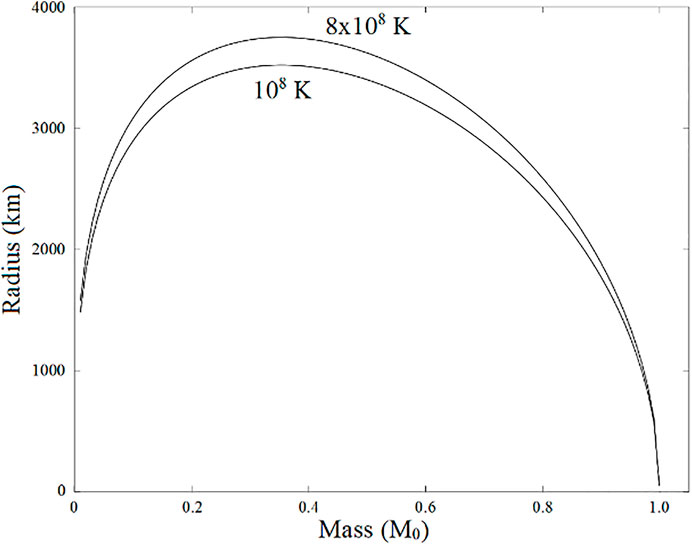
\frac{N}{V} ≫ \frac{8 π {(m_{e} c^{2})}^{3}}{3 h^{3}} = 5.2 \times 10^{35} e l e c t r o n s / m^{3} (52)

FIGURE 1

FIGURE 1. The relation between the radius and mass of the white dwarf star calculated by Eq. 49 at the condition p_F >> m_ec without considering the equations of hydrostatic equilibrium.

As long as the white dwarf star has the minimal density as shown in Eq. 51, this condition in Eq. 52 is automatically satisfied. In our common environment on the Earth, most things have density much lower than that of the white dwarf star in Eq. 51. When something disappears like the water evaporating, its volume will become larger and larger, and then, its density is closer and closer to zero. A white dwarf star with very large radius as its mass approaches zero is much unreasonable because it directly violates the criterion in Eq. 52 and our knowledge about the white dwarf star. The similar mass–radius relation trend has been shown in Figure 9 of the reference (Bvdard et al., 2017) where pure iron cores surrounded by helium and hydrogen layers are considered. Three demonstrations reveal arc curves whose maximum radii appearing at mass M between $0.40$ and $0.55 M_{⊙}$ , and then, the radii in these three cases are all decreased when the mass of the white dwarf star is below maximum (Bédard et al., 2017). Even for the C/O-core model, a core consisting of a uniform mixture of carbon and oxygen in equal proportions, the mass–radius relations of three different temperatures all show gradual decrease below $M = 1.10 M_{⊙}$ (Bédard et al., 2017). Another similar mass–radius trend at the low-mass region is shown in Figure 2 of the reference (Nunes et al., 2021) where it clearly exhibits all five temperature cases, leading to the radial coordinate R→0 at the mass of the white dwarf star M→0. This result supports our above statements that the radius of the white dwarf star is close to zero when its mass approaches zero. The zero-mass thing shall occupy no volume in space, not to be a sphere with a divergent radius. On the other hand, although our calculations do not have relation with the magnetic field, it is still worthy to mention that some recent research also show the radius of the highly magnetized white dwarf star approaching zero at their mass M close to zero (Das and Mukhopadhyay, 2012; Kundu and Mukhopadhyay, 2012; Das and Mukhopadhyay, 2013). This kind of the strongly magnetic white dwarf star has the strong magnetic field about 10¹⁵–10¹⁷ G at the center (Das and Mukhopadhyay, 2012) and may explain the origin of overluminous peculiar type Ia supernova. The research of the strongly magnetic carbon–oxygen white dwarf star exhibits the mass–radius relation in Figure 2 (Kundu and Mukhopadhyay, 2012) where the Chandrasekhar mass limit is exceeded and the generic mass limit is proposed to be $2.58 M_{⊙}$ . The mass–radius relations in Figures 2 and 3 of the reference (Das and Mukhopadhyay, 2012) are shown for one-level, two-level, and three-level systems. The curve of the one-level system is single-valued, but one mass corresponds to three radii at most for the two-level system and four radii at most for the three-level system (Das and Mukhopadhyay, 2012). All curves also exhibit radii close to zero at mass M approaching zero. Usually speaking, the lower level system corresponds to the higher magnetic field at the center, and the larger Fermi energy has the higher magnetic field at the center (Das and Mukhopadhyay, 2012). For example, the central magnetic field is 6.6 × 10¹³ G at E_F = 2m_ec² for the one-level system, but it is as high as 8.82 × 10¹⁷ G at E_F = 200 m_ec² for the same system (Das and Mukhopadhyay, 2012). The higher-level mass–radius relation trend is much different from the non-magnetic white dwarf stars that we discuss in this manuscript. In addition, Figure 3 of the reference (Das and Mukhopadhyay, 2013) also show the mass–radius relations of the magnetic white dwarf stars for one-level systems where all the radii approach zero as their mass are close to zero. By the way, it also points out that the peculiar type Ia supernovae SN 2003fg, SN 2006gz, SN 2007if, and SN 2009dc may have super-Chandrasekhar mass limit of up to 2.4–2.8 $M_{⊙}$ (Das and Mukhopadhyay, 2012). Furthermore, the stability of such strongly magnetic white dwarf stars has also been discussed (Xhamel et al., 2013).

FIGURE 2

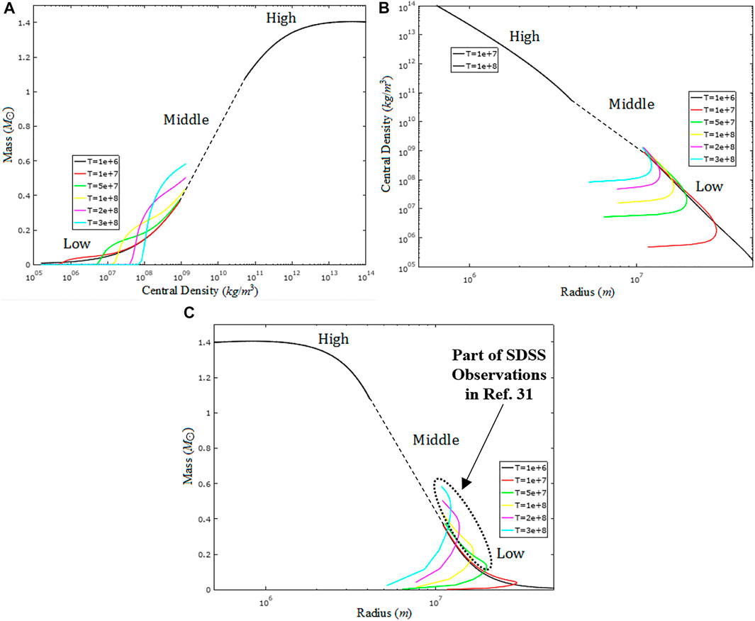
FIGURE 2. The relations at different temperature in the high-, middle-, and low-density regions between (A) mass and the central density, (B) the central density and radius, and (C) mass and radius. All the above results are obtained by considering the equations of hydrostatics equilibrium.

Another thing that we have to notice is the radius of the white dwarf star at its mass close to the upper mass limit. The mass–radius relation trends of most research and textbooks (Huang, 1987; Greiner et al., 1995; Carroll and Ostlie, 2006; Parsons et al., 2010; De Carvalho et al., 2014; Hermes et al., 2014; Franzon and Schramm, 2015; Bera and Bhattacharya, 2016; Boshkayev et al., 2016; Parsons et al., 2017; Sahu et al., 2017; Tremblay et al., 2017; Nunes et al., 2021) including ours all predict a zero radius when the mass is equal to the Chandrasekhar mass limit. However, it belongs to the black hole category, so we have to define a lower radius limit when the mass is close to M₀. Because we consider a non-rotating and non-charged white dwarf star, this lower radius limit is the Schwarzschild radius, which is GM₀/c² = 4.25 km for M₀ = $1.44 M_{⊙}$ .

The other consideration is about m_ec²>>E_F for the non-relativistic case, then the partition function, pressure, and number of the ideal Fermi electron gas become

\ln Z \approx g \frac{4 π V {(2 m_{e})}^{3 / 2}}{3 h^{3} β^{3 / 2}} \times [Γ (\frac{5}{2}) f_{5 / 2} (z) + \frac{3}{4} (\frac{k_{B} T}{m_{e} c^{2}}) Γ (\frac{7}{2}) f_{7 / 2} (z) + \frac{3}{32} {(\frac{k_{B} T}{m_{e} c^{2}})}^{2} Γ (\frac{9}{2}) f_{9 / 2} (z)], (53)

P_{e l e c t r o n g a s} \approx \frac{8 π {(2 m_{e})}^{3 / 2} {(k_{B} T)}^{5 / 2}}{3 h^{3}} [Γ (\frac{5}{2}) f_{5 / 2} (z) + \frac{3}{4} (\frac{k_{B} T}{m_{e} c^{2}}) Γ (\frac{7}{2}) f_{7 / 2} (z)], (54)

and

N (T, V, z) \approx \frac{4 π V {(2 m_{e})}^{\frac{3}{2}} {(k_{B} T)}^{3 / 2}}{h^{3}} \times [Γ (\frac{3}{2}) f_{3 / 2} (z) + \frac{5}{4} (\frac{1}{m_{e} c^{2} β}) Γ (\frac{5}{2}) f_{5 / 2} (z) + \frac{7}{32} {(\frac{1}{m_{e} c^{2} β})}^{2} Γ (\frac{7}{2}) f_{7 / 2} (z)] (55)

Combining Eq. 55 with Eq. 54, it gives the relation between P_{electron gas}, T, V, and N

P_{e l e c t r o n g a s} \approx \frac{2 N k_{B} T}{3 V} [\frac{Γ (\frac{5}{2}) f_{5 / 2} (z) + \frac{3}{4} (\frac{k_{B} T}{m_{e} c^{2}}) Γ (\frac{7}{2}) f_{7 / 2} (z) + \frac{3}{32} {(\frac{k_{B} T}{m_{e} c^{2}})}^{2} Γ (\frac{9}{2}) f_{9 / 2} (z)}{Γ (\frac{3}{2}) f_{3 / 2} (z) + \frac{5}{4} (\frac{k_{B} T}{m_{e} c^{2}}) Γ (\frac{5}{2}) f_{5 / 2} (z) + \frac{7}{32} {(\frac{k_{B} T}{m_{e} c^{2}})}^{2} Γ (\frac{7}{2}) f_{7 / 2} (z)}] (56)

Here, we use the non-relativistic chemical potential for E_F >> k_BT (Honerkamp, 2002)

μ \approx E_{F} [1 - \frac{π^{2}}{12} {(\frac{k_{B} T}{E_{F}})}^{2} - \frac{7 π^{4}}{640} {(\frac{k_{B} T}{E_{F}})}^{4}] (57)

where

E_{F} \approx \frac{p_{F}^{2}}{2 m_{e}} - \frac{p_{F}^{4}}{8 m_{e}^{3} c^{2}} (58)

Further rearrangement of Eq. 56 and ignoring T² terms in Eq. 56 and T⁴ term in Eq. 57 give

\begin{array}{l} P_{\begin{matrix} e l e c t r o n & g a s \end{matrix}} \approx \frac{2 N k_{B} T}{3 V} [\frac{Γ (\frac{5}{2}) f_{5 / 2} (z)}{Γ (\frac{3}{2}) f_{3 / 2} (z)}] {\frac{1 + \frac{3}{4} (\frac{k_{B} T}{m_{e} c^{2}}) [\frac{Γ (\frac{7}{2}) f_{7 / 2} (z)}{Γ (\frac{5}{2}) f_{5 / 2} (z)}]}{1 + \frac{5}{4} (\frac{k_{B} T}{m_{e} c^{2}}) [\frac{Γ (\frac{5}{2}) f_{5 / 2} (z)}{Γ (\frac{3}{2}) f_{3 / 2} (z)}]}} \approx \frac{N k_{B} T}{V} (\frac{2}{5} \ln z) [1 - \frac{3}{14} (\frac{k_{B} T}{m_{e} c^{2}} \ln z)] \\ \approx \frac{N}{V} {\frac{2}{5} E_{F} [1 - \frac{π^{2}}{12} {(\frac{k_{B} T}{E_{F}})}^{2}]} {1 - \frac{3}{14} (\frac{E_{F}}{m_{e} c^{2}}) [1 - \frac{π^{2}}{12} {(\frac{k_{B} T}{E_{F}})}^{2}]} \end{array} (59)

After obtaining the pressure of the ideal Fermi electron gas varying with temperature, then we can estimate the relation between mass and radius of the white dwarf star. The equilibrium condition in Eq. 43 becomes

(\frac{8 π m_{e}^{3} c^{3}}{3 h^{3}}) {\frac{2}{5} E_{F} [1 - \frac{π^{2}}{12} {(\frac{k_{B} T}{E_{F}})}^{2}]} \times {1 - \frac{3}{14} (\frac{E_{F}}{m_{e} c^{2}}) [1 - \frac{π^{2}}{12} {(\frac{k_{B} T}{E_{F}})}^{2}]} \frac{\bar{M}}{{\bar{R}}^{3}} = K^{'} \frac{{\bar{M}}^{2}}{{\bar{R}}^{4}}, (60)

and then it gives

M = (\frac{3}{2 δ G m_{n}}) {\frac{2}{5} E_{F} [1 - \frac{π^{2}}{12} {(\frac{k_{B} T}{E_{F}})}^{2}]} \times {1 - \frac{3}{14} (\frac{E_{F}}{m_{e} c^{2}}) [1 - \frac{π^{2}}{12} {(\frac{k_{B} T}{E_{F}})}^{2}]} R (61)

This reasonably shows that the radius disappears as M→0 verifying the previous viewpoint that zero mass represents no occupation or zero radius. However, the previous result shows the divergence of radius at M→0 (Carroll and Ostlie, 2006), and the mass–radius relation is

R \approx \frac{{(18 π)}^{2 / 3}}{10} \frac{ℏ^{2}}{G m_{e} M^{1 / 3}} {[(\frac{Z}{A}) \frac{1}{m_{n}}]}^{5 / 3}, (62)

where Z and A are the number of protons and nucleons, respectively. This expression is very problematic because the pressure is close to zero as R→∞ which can be seen directly from Eq. 59 that p is proportional to the inverse volume of the star or ∝ 1/R³. As we know, the pressure inside the white dwarf star is much higher than it is inside the Sun. The zero pressure inside the white dwarf star cannot satisfy the criteria in Eq. 52. When the pressure is close to zero everywhere, it cannot support a stable star anymore and the white dwarf star disappears at this zero-density and zero-pressure limit situation. Therefore, it is incorrect that the radius of the white dwarf star is divergent when its mass goes to zero. Besides, in Figure 6 of the reference (De Carvalho et al., 2014), the pressure in ¹²C white dwarf star decreases from 10²² to 10¹⁶ erg/cm³ when the density decreases from 5 × 10⁶ to 2 × 10² g/cm³. Theoretically speaking, when its density goes to zero, the pressure must approach zero. If the pressure is not zero but the density is zero at some temperatures (De Carvalho et al., 2014), then the calculations shall have some problem. A white dwarf star with a very large radius when its mass goes to zero is much unreasonable because it directly violates the criterion in Eq. 52 and our knowledge about the white dwarf star. In addition, as mentioned before, another similar mass–radius relation trend at the low-mass region clearly exhibits in Figure 2 of the reference (Nunes et al., 2021) that all five temperature cases lead to the radial coordinate R→0 as the mass of the white dwarf star M→0. This result supports our prediction given in Eq. 61 where R→0 at M→0. In summary, both the relativistic and non-relativistic electron gases lead to zero radius at M approaching zero, which correct the divergent result in the old $R \propto M^{- 1 / 3}$ .

The Mass–Radius Relation Obtained by Considering the Equations of Hydrostatic Equilibrium

Next, we further obtain some relations from the equation of hydrostatic equilibrium for the stellar structure in the Tolman–Oppenheimer–Volkoff (TOV) form (Koester and Chanmugam, 1990; De Carvalho et al., 2014; Boshkayev et al., 2016; Carvalho et al., 2018). There are two equations in TOV considered here without the correction 1/c² terms (Boshkayev et al., 2016):

\frac{d P (r)}{d r} = - \frac{G m (r) ρ (r)}{r^{2}} (63)

and

\frac{d m (r)}{d r} = 4 π r^{2} ρ (r), (64)

where p(r), m(r), and ρ(r) are the distributions of the pressure, mass, and mass density varying with the radial position in the star, respectively. This ignorance of the 1/c² terms makes us pay more attention to the dominant terms. Theoretically speaking, once the distribution of ρ(r) is known, the distributions of the pressure and mass can be obtained by substituting ρ(r) into Eqs. 63 and 64. The boundary conditions are m (0) = 0, ρ(0) = ρ_c, m (R⁺) = ρ(R⁺) = 0, and dρ(r)/dr = 0 at r = 0 where ρ_c is the central density. Two boundary conditions of m (0) = 0 at the center and p (R⁺) = 0 have been introduced in the paper (Koester and Chanmugam, 1990; Carvalho et al., 2018; Nunes et al., 2021). Then, defining a parameter

x = x_{F} \equiv \frac{p_{F}}{m_{e} c} = {(\frac{ρ}{ρ_{0}})}^{1 / 3}, (65)

where

ρ_{0} = 2 m_{n} (\frac{8 π m_{e}^{3} c^{3}}{3 h^{3}}), (66)

Using this parameter in Eq. 65, the high Fermi-energy pressure in Eq. 40 becomes

P_{e l e c t r o n g a s} \approx \frac{2 π m_{e}^{4} c^{5}}{3 h^{3}} x^{4} {[1 + \frac{1}{2} {(\frac{1}{x})}^{2} - \frac{π^{2}}{3} {(\frac{k_{B} T}{m_{e} c^{2}})}^{2} {(\frac{1}{x})}^{2}] - \frac{[\frac{3}{2} - π^{2} {(\frac{k_{B} T}{m_{e} c^{2}})}^{2}]}{[x^{2} - x + \frac{1}{2} - \frac{π^{2}}{3} {(\frac{k_{B} T}{m_{e} c^{2}})}^{2}]} + \frac{[3 - π^{2} {(\frac{k_{B} T}{m_{e} c^{2}})}^{2}] x}{{[x^{2} - x + \frac{1}{2} - \frac{π^{2}}{3} {(\frac{k_{B} T}{m_{e} c^{2}})}^{2}]}^{2}}} (67)

From Eq. 63, it leads

\frac{d ρ}{d r} = - {(\frac{d P}{d ρ})}^{- 1} \frac{G m ρ}{r^{2}} (68)

Then, it results in

\frac{d P}{d ρ} = (\frac{2 π m_{e}^{4} c^{5}}{3 h^{3}}) \frac{1}{3 ρ_{0}} {4 x + x - \frac{2 π^{2}}{3} {(\frac{k_{B} T}{m_{e} c^{2}})}^{2} x - [\frac{3}{2} - π^{2} {(\frac{k_{B} T}{m_{e} c^{2}})}^{2}] \frac{4 x}{x^{2} - x + \frac{1}{2} - \frac{π^{2}}{3} {(\frac{k_{B} T}{m_{e} c^{2}})}^{2}} + [\frac{3}{2} - π^{2} {(\frac{k_{B} T}{m_{e} c^{2}})}^{2}] \frac{x^{2} (2 x - 1)}{{[x^{2} - x + \frac{1}{2} - \frac{π^{2}}{3} {(\frac{k_{B} T}{m_{e} c^{2}})}^{2}]}^{2}} + [3 - π^{2} {(\frac{k_{B} T}{m_{e} c^{2}})}^{2}] \frac{5 x^{2}}{{[x^{2} - x + \frac{1}{2} - \frac{π^{2}}{3} {(\frac{k_{B} T}{m_{e} c^{2}})}^{2}]}^{2}} - [3 - π^{2} {(\frac{k_{B} T}{m_{e} c^{2}})}^{2}] \frac{2 x^{3} (2 x - 1)}{{[x^{2} - x + \frac{1}{2} - \frac{π^{2}}{3} {(\frac{k_{B} T}{m_{e} c^{2}})}^{2}]}^{3}}} (69)

Finally, we can obtain the differential equation of ρ(r) by substituting Eq. 69 into Eq. 68. Similarly, the case for the low Fermi-energy pressure can be obtained by using Eq. 56. For μ≥k_BT,

\frac{d P}{d ρ} = \frac{d}{d x} {(\frac{2 π m_{e}^{4} c^{5}}{3 h^{3}}) \frac{4}{5} (x^{5} - \frac{x^{7}}{4}) [1 - \frac{π^{2}}{3} {(\frac{k_{B} T}{m_{e} c^{2}})}^{2} \frac{1}{{(x^{2} - x^{4} / 4)}^{2}}] \times \frac{[y^{2} + \frac{5 π^{2}}{8} y^{4}] + \frac{15}{28} (\frac{k_{B} T}{m_{e} c^{2}}) [y + \frac{35 π^{2}}{24} y^{3}] + \frac{1}{48} {(\frac{k_{B} T}{m_{e} c^{2}})}^{2} [1 + \frac{21 π^{2}}{8} y^{2}]}{[y^{2} + \frac{π^{2}}{8} y^{4}] + \frac{3}{4} (\frac{k_{B} T}{m_{e} c^{2}}) [y + \frac{5 π^{2}}{8} y^{3}] + \frac{1}{16} {(\frac{k_{B} T}{m_{e} c^{2}})}^{2} [1 + \frac{35 π^{2}}{24} y^{2}]}} \frac{d x}{d ρ}, (70)

where

y \equiv \frac{k_{B} T}{μ}, (71)

and the expression of μ in Eq. 57 is adopted here. Using Eqs. 64 and 68 with the boundary conditions ρ(0) = ρ_c, ρ(R⁺) = 0, and dρ/dr = 0 at r = 0, we can obtain the central density–mass, central density–radius, and mass–radius relations numerically. The numerical method is the fourth-order Runge–Kutta method (Nakamura, 1995). According to the definition of the parameter x in Eq. 65, the calculations are divided into three regions by considering the central mass density ρ_c at different temperature. The temperature of the white dwarf star is considered homogeneously here. The high-density region is for ρ_c > ρ₀, and we choose ρ_c ≥ 5 × 10¹⁰ kg/m³ in our high-density calculations by using Eqs. 67 and 69. The low-density region is for ρ_c < ρ, and we choose ρ_c ≤ 10⁹ kg/m³ in the low-density calculations by using Eqs. 56 and 70. Between 10⁹ kg/m³ and 5 × 10¹⁰ kg/m³ is the middle-density region, where it can be approximated by connecting the high- and low-density regions directly. In Figure 2A, the relation between mass and the central density of the white dwarf star is given in the high-, middle-, and low-density regions at different temperature. In the high-density region, the mass is close to 1.4 M_⊙ after 10¹³ kg/m³. Those curves are almost the same one from low temperature to 10⁸ K in this region, so only two cases at 10⁷ K and 10⁸ K are shown. In the low-density region, those curves have tiny deviations until T = 10⁷ K, and especially, they are almost coincident at ρ_c ≥ 2 × 10⁷ kg/m³. At T = 5 × 10⁷ K, the curve is explicitly changed, and the starting point is at 5 × 10⁶ kg/m³. It means that the white dwarf star at this temperature has a central density higher than 5 × 10⁶ kg/m³. As temperature increases, the starting point of the central density also increases. It is about 10⁷ kg/m³ at 10⁸ K, 4 × 10⁷ kg/m³ at 2 × 10⁸ K, and 7 × 10⁷ kg/m³ at 3 × 10⁸ K. In the middle-density region, although the central density is only from 10⁹ kg/m³ to 5 × 10¹⁰ kg/m³, the range of mass covers a large interval from 0.4 M_⊙ to 1.1 M_⊙. It means that a large part of the white dwarf stars are in this region.

In Figure 2B, the relation between the central density and mass is given in the high-, middle-, and low-density regions at different temperature. Both axes are shown in log scale. The central density is from 10⁵ kg/m³ to 10¹⁴ kg/m³, and the radius is from 5 × 10⁵ to 5 × 10⁷. At 10⁶ K, it shows a logarithm relation between the central density and the radius of the white dwarf star. The higher central density is, the smaller the radius is. However, the trend is broken at 10⁷ K and above. At 10⁷ K, there is a turning point around the central density of 10⁶ kg/m³, which means that the maximal radius of the white dwarf star at this temperature is less than 3 × 10⁷ m or 3 × 10⁴ km. This turning point also means that the radius of the white dwarf star cannot increase infinitely as mentioned in Eq. 62. When the mass goes to zero, the radius also approaches zero. If we extend the curve to zeros radius, then it exhibits that the central density is always above 10⁵ kg/m³ at 10⁷ K. The turning point increases in the central density as temperature increases, but the maximal radius decreases at the same time. The turning point is roughly 10⁷ kg/m³ at 5 × 10⁷ K and 10⁸ kg/m³ at 2 × 10⁸ K. In conclusion, the same radius of the white dwarf star would correspond to different central density, and one is in the high-density region and the other is in the low-density region.

In Figure 2C, the mass–radius relation for the white dwarf star is shown. As mentioned in Figure 2A, the mass is close to 1.4 M_⊙ after 10¹³ kg/m³ in the high-density region. Those curves are almost the same one from low temperature to 10⁸ K in the high-density region, and only two cases at 10⁷ K and 10⁸ K are shown in this region. In the low-density region, those curves have tiny deviations until T = 10⁷ K, and it is almost coincident at ρ_c ≥ 2 × 10⁷ kg/m³. In the middle-density region, the range of mass covers a large interval from 0.4 to 1.1 M_⊙ where the central density is only from 10⁹ kg/m³ to 5 × 10¹⁰ kg/m³. It also implies that a large part of the white dwarf stars that we found astronomically belong to the middle-density region. Those results are the same as Figure 2A. Especially, at T = 5 × 10⁷ K and above, there exist some parts where the mass at the same radius is larger than the curve at 10⁷ K and below. Recently, the Sloan Digital Sky Survey Release 4 shows a lot of observations having larger mass compared to the relativistic EOS at T = 0 K when the radius is larger than 8 × 10³ km (De Carvalho et al., 2014). By using our calculations in Figure 2C, this phenomenon can be explained because the higher temperature results in these white dwarf stars with larger mass appearing at the same radius in the low-density region. Usually, the temperature of these white dwarf stars is higher than 10⁷ K. Those parts are denoted by the dotted elliptic curve in Figure 2C. This explanation can also extend to the middle region in Figure 2C.

Compare Figure 2C with Figure 1, both mass–radius relation trend is similar for T > 0. We can find that all cases show the maximum radii appearing between 0 and $1.4 M_{⊙}$ . In addition, as mentioned previously, the similar mass–radius relation trend has been shown in Figure 9 of the reference (Bédard et al., 2017) where pure iron cores surrounded by helium and hydrogen layers are considered. Three demonstrations reveal arc curves whose maximum radii appearing at mass M between $0.40$ and $0.55 M_{⊙}$ , and then, the radii in these three cases are all decreased when the mass of the white dwarf star is below maximum (Bédard et al., 2017). Even for the C/O-core model, a core consisting of a uniform mixture of carbon and oxygen in equal proportions, the mass–radius relations of three different temperatures all show gradual decrease below M = 1 $.10 M_{⊙}$ (Bédard et al., 2017).

Conclusion

In summary, the mass–radius relation of the white dwarf star derived according to statistical mechanics shows that the temperature effect has to be considered at high temperature above 10⁷ K. After all, the ideally degenerate Fermi electron gas is described at T = 0 K, and the temperature effect would show something difference. The other correction is due to the electron–electron interaction considered at T = 0. The calculation considers the relativistic electrons, and the result shows that this effect causes the pressure 2/137 time less than the original value. It means that the many-particle effect appears and causes about 1.5% deviation in pressure. When the temperature effect is considered, the pressure is calculated by statistical mechanics. According to the Fermi energy, two cases are calculated. One is E_F >> m_ec² for the relativistic case, and the other is E_F << m_ec² for the non-relativistic case. Because of the temperature effect, the chemical potential is also temperature-dependent and different expression in these two cases. From the deductions, the pressure produced by the Fermi electron gas depends on temperature complicatedly at the given particle number N and volume V. Traditional formula gives the problematic relation $R \propto M^{- 1 / 3}$ because it leads to R→∞ and p→0 as M→0. Therefore, we correct this relation and obtain two much reasonable relations in the relativistic and nonrelativistic regions. The mass–radius relation of the white dwarf star without considering the equations of hydrostatic equilibrium is obtained for the relativistic and non-relativistic cases in which the radius is shown to be zero as the mass of the white dwarf star disappears.

Then, further considering the equations of hydrostatic equilibrium, the central density–mass, the central density–radius, and the mass–radius relations are obtained. The central density is divided into the high-, middle-, and low-density regions where the results can be coincident with the SDSS observations. In the high-density region, three relations are almost unchanged until 10⁸ K. The temperature effect mainly affects the low-density region at temperature above 10⁷ K. Especially, the mass–radius curves show some parts having larger mass at the same radius when temperature is higher. It gives a way to explain the SDSS observations at the radius more than 8 × 10³ km that the mass of the white dwarf star is often larger than the prediction by the relativistic EOS at zero temperature. Those white dwarf stars of larger mass just correspond to the low- and middle-density regions. It means that we should consider the temperature effect to get better calculations that can reasonably explain the astronomical observations. Although the temperature is maximum at the center and minimum at the surface in reality, we still adopt the uniform temperature approximation as most research did. Our results imply that the uniform temperature approximation may remain valuable. Furthermore, the temperature can change with time because the white dwarf stars cool down by thermal emission. However, the cooling time is much longer than the astronomical observations, the temperature of the white dwarf star is kept constant at each calculation in our research. It is a good enough way to hold the initial temperature throughout each calculation if we want to compare the calculation results with the astronomical observations in several decades.

Data Availability Statement

The raw data supporting the conclusion of this article will be made available by the authors, without undue reservation.

Author Contributions

The single author first reads a lot of references to propose this research idea. Then, he carefully derives all the mathematical equations in this manuscript and checks them several times. He also writes down the programs to calculate some examples to demonstrate the concepts revealing in this manuscript. After obtaining some results, he starts to write this paper and finishes it. Finally, he prepares this paper and submits it.

Conflict of Interest

The author declares that the research was conducted in the absence of any commercial or financial relationships that could be construed as a potential conflict of interest.

Publisher’s Note

All claims expressed in this article are solely those of the authors and do not necessarily represent those of their affiliated organizations or those of the publisher, the editors, and the reviewers. Any product that may be evaluated in this article, or claim that may be made by its manufacturer, is not guaranteed or endorsed by the publisher.

Acknowledgments

The author thanks the Institute of Astronomy and Astrophysics at Academia Sinica in Taiwan for the financial support of this article. The author is also grateful to the reviewers for their comments to strengthen the statements in this article, and thankful to Dr. Ming-Jye Wang for his encouragement.

References

Bédard, A., Bergeron, P., and Fontaine, G. (2017). Measurements of Physical Parameters of White Dwarfs: A Test of the Mass-Radius Relation. Astrophys. J. 848, 11. doi:10.3847/1538-4357/aa8bb

CrossRef Full Text | Google Scholar

Bera, P., and Bhattacharya, D. (2016). Mass-radius Relation of Strongly Magnetized white Dwarfs: Dependence on Field Geometry, GR Effects and Electrostatic Corrections to the EOS. Mon. Not. R. Astron. Soc. 456, 3375–3385. doi:10.1093/mnras/stv2823

CrossRef Full Text | Google Scholar

Boshkayev, K. A., Rueda, J. A., Zhami, B. A., Kalymova, Z. A., and Balgymbekov, G. S. (2016). Equilibrium Structure of white Dwarfs at Finite Temperatures. Int. J. Mod. Phys. Conf. Ser. 41, 1660129. doi:10.1142/s2010194516601290

CrossRef Full Text | Google Scholar

Carroll, B. W., and Ostlie, D. A. (2006). An Introduction to Modern Astrophysics. 2nd ed. Addison-Wesley.

Google Scholar

Carvalho, G. A., Marinho, R. M., and Malheiro, M. (2018). General Relativistic Effects in the Structure of Massive White Dwarfs. Gen. Relativ Gravit. 50, 38. doi:10.1007/s10714-018-2354-8

CrossRef Full Text | Google Scholar

Chandrasekhar, S. (2012). An Introduction to the Study of Stellar Structure. Chicago: Dover.

Google Scholar

Chandrasekhar, S. (1935). The Highly Collapsed Configurations of a Stellar Mass. (Second Paper.). Mon. Not. R. Astron. Soc. 95, 207–225. doi:10.1093/mnras/95.3.207

CrossRef Full Text | Google Scholar

D’antonia, F., and Mazzitelli, I. (1990). Cooling of White Dwarfs. Annu. Rev. Astron. Astrophysics 28, 139.

Google Scholar

Das, U., and Mukhopadhyay, B. (2013). New Mass Limit for white Dwarfs: Super-chandrasekhar Type Ia Supernova as a New Standard Candle. Phys. Rev. Lett. 110, 071102. doi:10.1103/PhysRevLett.110.071102

PubMed Abstract | CrossRef Full Text | Google Scholar

Das, U., and Mukhopadhyay, B. (2012). Strongly Magnetic Cold Degenerate Electron Gas: Mass-Radius Relation of the Magnetized White Dwarfs. Phys. Rev. D 86, 042001. doi:10.1103/physrevd.86.042001

CrossRef Full Text | Google Scholar

De Carvalho, S. M., Rotondo, M., Rueda, Jorge. A., and Ruffini, R. (2014). The Relativistic Feynman-Metropolis-Teller Treatment at Finite Temperatures. Phys. Rev. C 89, 015801. doi:10.1103/physrevc.89.015801

CrossRef Full Text | Google Scholar

Soares, E. d. A. (2017). Constraining Effect Temperature, Mass and Radius of Hot White Dwarfs. arXiv preprint arXiv:1701.02295.

Google Scholar

Franzon, B., and Schramm, S. (2015). Effects of strong Magnetic fields and Rotation on white dwarf Structure. Phys. Rev. D 92, 083006. doi:10.1103/physrevd.92.083006

CrossRef Full Text | Google Scholar

Gasiorowicz, S. (1974). Quantum Physics. Singapore: Joh Wiley & Sons, Inc., 185.

Google Scholar

Gottfried, K., and Yan, T.-M. (2003). Quantum Mechanics: Fuandamentals. 2nd ed. New York, NY: Springer, 235–266. Hydrogenic Atoms. doi:10.1007/978-0-387-21623-2_5

CrossRef Full Text | Google Scholar

Graham, W. (2000). The Cambridge Handbook of Physics Formulas. Cambridge: Cambridge University Press.

Google Scholar

Greiner, W., Ludwig, N., and Stocker, H. (1995). Thermodynamics and Statistical Mechanics. New York: Springer, 359.

Google Scholar

Hans, C. O., and Ruffini, R. (1994). Gravitation and Spacetime. 2nd ed. New York: W. W. Norton & Company.

Google Scholar

Hermes, J. J., Brown, W. R., Kilic, M., Gianninas, A., Chote, P., Sullivan, D. J., et al. (2014). Radius Constraints from High-Speed Photometry of 20 Low-Mass White Dwarf Binaries. ApJ 792, 39. doi:10.1088/0004-637x/792/1/39

CrossRef Full Text | Google Scholar

Holberg, J. B. (2005). How Degenerate Star Came to Be Known White Dwarf. Bull. Am. Astronomical Soc. 37, 1503.

Google Scholar

Honerkamp, J. (2002). Statistical Physics-An Advanced Approach with Applications. 2nd ed. Berlin Heidelberg: Springer, 233.

Google Scholar

Huang, K. (1987). Statistical Mechanics. 2nd ed. John Wiley & Sons, 247.

Google Scholar

Kepler, S. O., Kleinman, S. J., Nitta, A., Koester, D., Castanheira, B. G., Giovannini, O., et al. (2007). White Dwarf Mass Distribution in the SDSS. Mon. Not. R. Astron. Soc. 375, 1315–1324. doi:10.1111/j.1365-2966.2006.11388.x

CrossRef Full Text | Google Scholar

Kittel, C., and Kroemer, H. (1980). Thermal Physics. 2nd ed. San Francisco: W. H. Freeman and Company, 196.

Google Scholar

Koester, D., and Chanmugam, G. (1990). Physics of White Dwarf Stars. Rep. Prog. Phys. 53, 837–915. doi:10.1088/0034-4885/53/7/001

CrossRef Full Text | Google Scholar

Kundu, A., and Mukhopadhyay, B. (2012). Mass of Highly Magnetized White Dwarfs Exceeding the Chandrasekhar Limit: an Analytical View. Mod. Phys. Lett. A. 27, 1250084. doi:10.1142/s0217732312500848

CrossRef Full Text | Google Scholar

Levin, F. S. (2002). An Introiduction to Quantum Theory. Cambridge: Cambridge University Press, 421.

Google Scholar

Mahan, G. D. (2000). Many-particle Physics. 3rd ed. New York, NY: Kluwer Academic, 297.

Google Scholar

Mattuck, R. D. (1976). A Guide to Feynman Diagrams in the Many-Body Problem. 2nd ed. New York: Dover, 217.

Google Scholar

Misner, C. W., Thorne, K. S., and Wheeler, J. A. (2017). Gravitation. Princeton University Press.

Google Scholar

Mould, R. A. (2002). Basic Relativity. New York: Springer.

Google Scholar

Nakamura, S. (1995). Applied Numerical Methods in C. Simon & Schuster (Asia) Pte. Ltd., 332.

Google Scholar

Nunes, S. P., ArbañilArbañil, J. D. V., and Malheiro, M. (2021). The Structure and Stability of Massive Hot White Dwarfs. ApJ 921, 138. doi:10.3847/1538-4357/ac1e8a

CrossRef Full Text | Google Scholar

Parsons, S. G., Gänsicke, B. T., Marsh, T. R., Ashley, R. P., Bours, M. C. P., Breedt, E., et al. (2017). Testing the White Dwarf Mass-Radius Relationship with Eclipsing Binaries. Mon. Not. R. Astron. Soc. 470, 4473–4492. doi:10.1093/mnras/stx1522

CrossRef Full Text | Google Scholar

Parsons, S. G., Marsh, T. R., Copperwheat, C. M., Dhillon, V. S., Littlefair, S. P., Gänsicke, B. T., et al. (2010). Precise Mass and Radius Values for the white dwarf and Low Mass M dwarf in the Pre-cataclysmic Binary NN Serpentis. Mon. Not. R. Astron. Soc. 402, 2591–2608. doi:10.1111/j.1365-2966.2009.16072.x

CrossRef Full Text | Google Scholar

Roger, G. N. (2002). Quantum Physics. New York: Springer, 100.

Google Scholar

Sahu, K. C., Anderson, J., Casertano, S., Bond, H. E., Bergeron, P., Nelan, E. P., et al. (2017). Relativistic Deflection of Background Starlight Measures the Mass of a Nearby white dwarf star. Science 356, 1046–1050. doi:10.1126/science.aal2879

PubMed Abstract | CrossRef Full Text | Google Scholar

Salpeter, E. E. (1961). Energy and Pressure of a Zero-Temperature Plasma. ApJ 134, 669. doi:10.1086/147194

CrossRef Full Text | Google Scholar

Schutz, B. F. (1985). A First Course in General Relativity. Cambridge: Cambridge University Press, 266.

Google Scholar

Schwabl, F. (2002). Statistical Mechanics. Berlin Heidelberg: Springer, 184.

Google Scholar

Tremblay, P.-E., Gentile-Fusillo, N., Raddi, R., Jordan, S., Besson, C., Gänsicke, B. T., et al. (2017). TheGaiaDR1 Mass-Radius Relation for white Dwarfs. Mon. Not. R. Astron. Soc. 465, 2849–2861. doi:10.1093/mnras/stw2854

CrossRef Full Text | Google Scholar

Xhamel, N., Fantina, A. F., and Davis, P. J. (2013). Stability of Super-chanderasekhar Magnetic White Dwarfs. Phys. Rev. D 88, 081301. doi:10.1103/PhysRevD.88.081301

CrossRef Full Text | Google Scholar

Keywords: white dwarf star, degenerate Fermi electron gas, pressure, upper mass limit, electron–electron interaction

Citation: Pei T-H (2022) The Highly Accurate Relation Between the Radius and Mass of the White Dwarf Star From Zero to Finite Temperature. Front. Astron. Space Sci. 8:799210. doi: 10.3389/fspas.2021.799210

Received: 21 October 2021; Accepted: 08 December 2021;
Published: 01 February 2022.

Edited by:

Scott William McIntosh, National Center for Atmospheric Research (UCAR), United States

Reviewed by:

Kazuharu Bamba, Fukushima University, Japan
Herman J. Mosquera Cuesta, Tecnologia e Innovacion, Colciencias, Colombia

Copyright © 2022 Pei. This is an open-access article distributed under the terms of the Creative Commons Attribution License (CC BY). The use, distribution or reproduction in other forums is permitted, provided the original author(s) and the copyright owner(s) are credited and that the original publication in this journal is cited, in accordance with accepted academic practice. No use, distribution or reproduction is permitted which does not comply with these terms.

*Correspondence: Ting-Hang Pei, Thpei142857@gmail.com, thpei@asiaa.sinica.edu.tw

ORIGINAL RESEARCH article

The Highly Accurate Relation Between the Radius and Mass of the White Dwarf Star From Zero to Finite Temperature

Introduction

The Degenerate Fermi Electron Gas for the White Dwarf Star

The Correction of the Electron–Electron Interaction for the White Dwarf Star at T = 0

The Temperature Effect on the Pressure of the Ideal Fermi Electron Gas in the White Dwarf Star

The Mass–Radius Relation Obtained by Considering the Equations of Hydrostatic Equilibrium

Conclusion

Data Availability Statement

Author Contributions

Conflict of Interest

Publisher’s Note

Acknowledgments

References

People also looked at