 Lauren M. Fry
 Andrew D. Gronewold
 Frank Seglenieks
 Samar Minallah4
 Deanna Apps
- 1Great Lakes Environmental Research Laboratory, Office of Oceanic and Atmospheric Research, National Oceanic and Atmospheric Administration, Ann Arbor, MI, United States
- 2School for Environment and Sustainability, University of Michigan, Ann Arbor, MI, United States
- 3Environment and Climate Change Canada, Canadian Centre for Inland Waters, Burlington, ON, Canada
- 4Department of Climate and Space Sciences and Engineering, University of Michigan, Ann Arbor, MI, United States
- 5Hydraulics and Hydrology Branch, United States Army Corps of Engineers, Detroit, MI, United States
- 6Environment and Climate Change Canada, Great Lakes and St. Lawrence River Regulation Office, Cornwall, ON, Canada
Despite the fact that the Great Lakes contain roughly 20% of the world's surface freshwater, there is a relatively limited body of recent work in peer reviewed literature that addresses recent trends in lake levels. This work is largely coming from a handful of authors who are most well-versed in the complexities of monitoring and modeling in a basin that spans an international border and contains vast areas of surface water connected by both natural and managed connecting channel flows. At the same time, the recent dramatic changes from record low water levels in the early 2010's to record high water levels across the Great Lakes in 2019 and 2020 have brought significant attention to the hydroclimatic conditions in the basin, underscoring the need to bring new approaches and diverse perspectives (including from outside the basin) to address hydroclimate research challenges in the Great Lakes. Significant effort has led to advancements in data and model coordination among U.S. and Canadian federal agencies throughout the decades, and at the same time research from the broader community has led to higher resolution gridded data products. In this paper, we aim to present the current state of data and models for use in hydrological simulation with the objective of providing a guide to navigating the waters of Great Lakes hydroclimate data. We focus on data for use in modeling water levels, but we expect the information to be more broadly applicable to other hydroclimate research. We approach this by including perspectives from both the Great Lakes water management community and the broader earth science community.
Introduction
Anthropogenic climate change, population growth and the accompanying urbanization and agricultural demand, and economic development have been increasingly placing pressure on the world's freshwater (Wada et al., 2017). In addition, there is general agreement that intensification of the hydrologic cycle as a result of anthropogenic change means that assumptions of stationarity are not sufficient to inform water management. In the Great Lakes region, changes in the hydrologic cycle have been observed in the form of increasingly variable water levels (Gronewold and Rood, 2019). From the late 1990's to 2020, the Great Lakes have experienced both record low water levels, during an extended period of low water on Lake Superior and Lake Michigan-Huron, and record high water levels, following a dramatic multi-year rise culminating in record high water levels on all lakes in 2017, 2019, and/or 2020, depending on the lake. Adaptive management of Great Lakes water resources requires understanding and predicting changes in Great Lakes water balance components under a changing hydroclimate. The intensification of the hydrologic cycle, along with increasing pressure on Great Lakes water resources, motivates the need for advancing hydroclimate modeling in the Great Lakes basin.
Early development of Great Lakes basin runoff and evaporation models (Croley II, 1983, 1989) was arguably at the forefront of large scale hydrological modeling, and was driven largely by the need to understand and predict changes in Great Lakes water levels. Since then, significant advancements have been made in the arena of large basin, continental, and earth systems modeling and data due to water scarcity and flooding concerns (e.g., Salas et al., 2017; Xue et al., 2017; Lakshmi et al., 2018, among others).
Despite the growing body of research (and researchers) aimed at advancing large basin hydrological models, improvements to Great Lakes regional modeling have been limited. This is, in part, due to challenges related to identifying appropriate hydroclimate data sources for use in model development and simulation. Data discontinuities that result from both the international border and the vast surface area of the lakes themselves, where surface observations are scarce, pose unique challenges in hydroclimate data development and use (Gronewold et al., 2018). The authors of this article have observed that although there is significant effort put toward developing, compiling, and coordinating hydroclimate data across the border (Gronewold et al., 2018), there is a need to communicate these data to the broader hydroclimate and hydrological modeling communities. The objectives of this article are to (1) document the unique hydroclimate data requirements for Great Lakes hydrological modeling, and (2) direct the reader to readily available datasets coming from both the water management and numerical modeling communities that have been developed with these requirements in mind. Focus is geared toward datasets used for model development and historical simulation of water supply and water levels.
Resolving Earth Systems and Water Science Perspectives
Monitoring, forecasting, and managing Great Lakes water supplies and water levels requires complex, internationally-coordinated hydroclimate models and data sets. Nowhere else on Earth is there such a large chain of interconnected lakes (only Lake Baikal has a larger volume than the collective volume of the Great Lakes, and Lake Superior alone is the largest lake on Earth by surface area) and such a diverse range of thermodynamic behavior (including, for example, seasonal ice cover formation and the propagation of lake effect snow events). The challenges of developing and applying hydroclimate models and data to this massive freshwater system are further exacerbated by differences in federal agency monitoring protocols and modeling frameworks on either side of the U.S.-Canada international border. These differences can propagate into severe biases and anomalies in widely-distributed data products. For example, the National Oceanic and Atmospheric Administration (NOAA) National Center for Environmental Prediction North American Regional Reanalysis (NCEP-NARR) spatial patterns of precipitation and evaporation reveal dry conditions directly over the U.S.-Canada border. This is likely a result of the differences in observation datasets assimilated by NARR where a sharp contrast exists between the two countries, with considerable sparsity of surface observations incorporated by NARR over the Canadian side of the Great Lakes basin (Figure 1; Minallah and Steiner, 2021a).
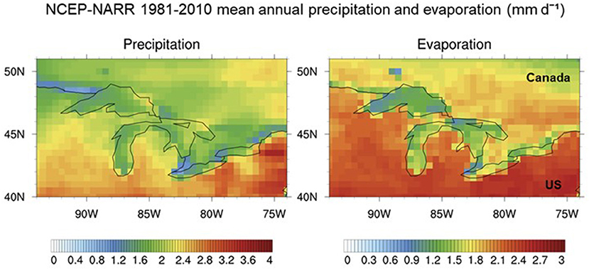
Figure 1. Visible discontinuities in (left) precipitation and (right) evaporation (evapotranspiration over the land surface) along the US-Canada border in the NCEP North American Regional Reanalysis.
In light of these challenges, it is the authors' belief that two distinct approaches to developing and applying Great Lakes hydroclimate data and models have evolved. A primary goal of this paper is to address and begin to reconcile those two approaches. The first approach directly embraces and responds to the needs of Great Lakes regional water resources management authorities. The second perspective is rooted in the historical and ongoing development of complex numerical models covering broad spatial domains that rely on explicit modeling of critical physical processes.
The regional water resources management perspective is largely driven by the mandate facing the three Great Lakes International Boards of Control, all of which operate under the auspices of the 1909 Boundary Waters Treaty and subsequent formation of the International Joint Commission, or IJC (Lemarquand, 1993). The three Boards work collectively to ensure that outflows from Lake Superior and Lake Ontario, as well as ice and flow control structures above Niagara Falls, are all operated in accordance with IJC regulation plans. The decisions made by these boards are guided by regulation plans and treaties that have been developed using historical records of incoming water supplies, connecting channel flows, and lake water levels. In addition, current conditions can act as triggers for decisions within the regulation plans. For example, the relative difference between the water levels of Lake Superior and Lake Michigan-Huron is one of the factors for how much water is released from Lake Superior.
Of course, having coordinated values of water levels, connecting channel flows, and historical water supply is crucial, as even differences of 1 cm in water level could result in different decisions being made. It is also imperative to coordinate values communicated to the public. This is especially critical during times of extreme conditions, when differing values could result in public confusion if mixed messages are received from the regulation agencies. Finally, coordinated historical datasets are an integral part of the process of developing and evaluating regulation plans, which includes examining the trends in water levels and their drivers.
The need for such tight coordination has led some of the management boards to form subcommittees that specifically look at these issues. For instance, the International Lake Ontario St. Lawrence River Board has granted authority to the St. Lawrence Committee on River Gauging to oversee and ensure the accuracy of flow estimates and water level measurements in the international section of the St. Lawrence River. This Committee inspects the computational methods and conducts an annual field inspection of the water level gages used by the Board to monitor river conditions and performs monthly audits of the water level and outflow data collected and archived by the power entities. In addition, the need to coordinate data to inform water management decisions on the Great Lakes led to the establishment of the Coordinating Committee for Great Lakes Basic Hydraulic and Hydrologic Data (subsequently referred to as “Coordinating Committee”) in 1953. This group, which consists of members from U.S. and Canadian federal agencies responsible for water balance monitoring, forecasting, and management, works to coordinate data required by the Boards of Control. Datasets that have been officially coordinated are in bold text in Tables 1–5. In addition to coordinating official datasets, the Coordinating Committee also serves as a forum for federal scientists and engineers to compile, understand, and evaluate recent advancements in available data products for all variables of the water balance.
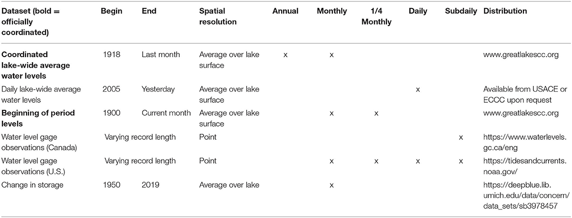
Table 1. Water level data products.
While the models and data sets used by the Boards of Control (and other regional management authorities) were developed by scientists and practitioners with this “first” perspective and explicitly include local-scale hydroclimate phenomena and anthropogenic impacts on the hydrology cycle, they typically do not adequately reflect climatological dynamics at regional to continental scales, nor do they typically reflect broad advancements in the state-of-the-art in hydroclimate modeling.
The second perspective on the development of Great Lakes hydroclimate models and data is, in fact, directly aligned with the earth systems modeling community. Numerical earth systems models require spatially consistent data spanning regional to global areas. Although this perspective does not conflict with the water management perspective, we find that there is significant room for improving the integration of research advances by the earth systems modeling community, and likewise improving the application of advancements in Great Lakes region specific data resulting from collaborations in the Water Management arena. This paper represents a step toward reconciling these two approaches.
Summary of Available Datasets and Conventional Applications
The following subsections describe datasets for each variable of the Great Lakes water balance, shown in Equation (1). Datasets are summarized in Tables 1–5.
where dS is the change in storage (i.e., the change in volume due to changes in lake level), Qin is the inflow from the upstream lake and through diversions as described in Section Diversion Flows, Qout is the outflow to the downstream lake (or, in the case of Lake Ontario, to the St. Lawrence River) and through diversions as described in Diversion Flows, P is the precipitation falling directly over the lake surface, R is the lateral tributary runoff into the lake, E is the evaporation from the lake surface, and ε is the uncertainty term. Conventional practice is to lump direct groundwater inflow and thermal expansion into this uncertainty term.
Water Levels
Water level data products are shown in Table 1. For the purpose of monitoring and predicting the water budget of the Great Lakes, officially coordinated water levels are computed as lake-wide averages. Also, since Lake Michigan and Lake Huron are connected via the Straits of Mackinac, hydrologically they are considered one lake, referenced as “Lake Michigan-Huron.” Lake-wide average water levels are calculated using a network of gages that has been agreed upon by the Coordinating Committee to give a complete depiction of the water level across the entire lake surface. Lake-wide average levels have been computed using a different set of gages over time on each lake due to data availability dating back to the 1860's. The gages listed below are the locations included in lake-wide average water level calculations currently:
Lake Superior: Point Iroquois, Michipicoten, Thunder Bay, Marquette, and Duluth
Lake Michigan-Huron: Harbor Beach, Thessalon, Mackinaw City, Milwaukee, Ludington, Tobermory
Lake St. Clair: Belle River and St. Clair Shores
Lake Erie: Port Colborne, Port Stanley, Toledo, Cleveland
Lake Ontario: Oswego, Toronto, Kingston, Rochester, Port Weller, Cobourg.
The U.S. locations are gages operated by the National Oceanic and Atmospheric Administration (NOAA) and the gages in Canada are operated by the Canadian Hydrographic Service (CHS).
Officially coordinated monthly mean (MM) lakewide average water levels are computed using the same procedure by both the U.S. Army Corps of Engineers (USACE) and Environment and Climate Change Canada (ECCC): (1) compute daily means for each gage and round to the nearest 0.01 m, (2) compute the lakewide average (using gage pairing logic described in Supplementary Tables 1–5 when a gage is missing daily data) and round to the nearest 0.01 m, (3) compute monthly mean lakewide average water levels by taking the mean daily values for each day in the month and round to the nearest 0.01 m. The same procedure is used to compute beginning of month water levels, except that in the third step, the beginning of month (BOM) level is computed by taking the average of the daily lakewide average water level on the last day of the month just ending and the 1st day of the month just starting for each lake. Coordinated BOM and MM water levels are significant data for use in outflow management, as described in Section Resolving Earth Systems and Water Science Perspectives. Accordingly, considerable attention is given to ensuring that both agencies use the same procedure, including the rounding. For each rounding application, the practice is to round to the nearest even centimeter when the thousandth of a meter is 5 (National Aeronautics Space Administration, 1994). For example, if the water level is 183.565 m, the rounded water level would be rounded to 183.56 m.
MM water levels and BOM levels are coordinated between federal agencies in both the U.S. and Canada. Those agencies are the USACE and ECCC. At the end of every month, MM and BOM levels are preliminarily coordinated as part of operational forecasting procedures. In the spring, when daily water level data has been verified by NOAA and CHS through December of the previous year, final coordination is done for all months of the year that just ended. MM water levels as of September 2021 are shown in Figure 2, with 2021 data still provisional. Data for the full coordinated period of record back to 1918 can be obtained from the Coordinating Committee.
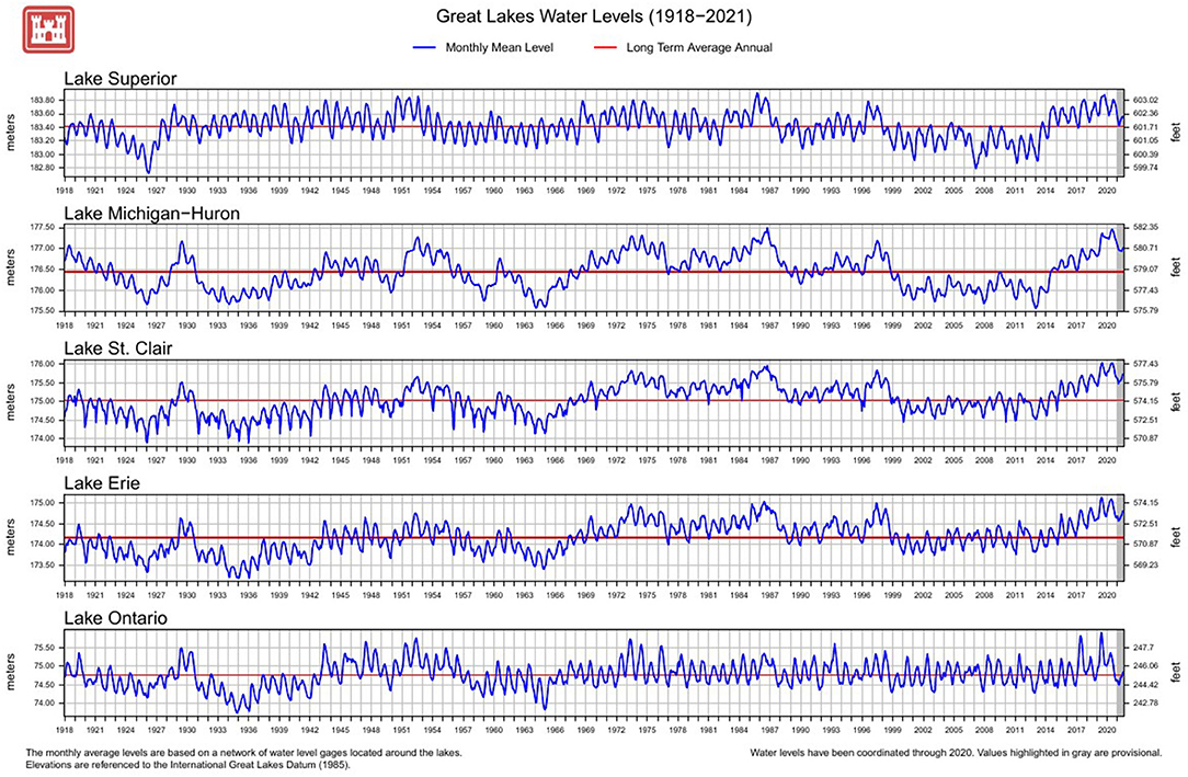
Figure 2. Monthly mean water levels for each of the Great Lakes and Lake St. Clair shown as a blue line (as of September 2021). 2021 data highlighted in gray is still provisional (source: www.lre.usace.army.mil).
Water levels are measured as a surface elevation with reference to the International Great Lakes Datum (IGLD) 1985. The IGLD 1985 reference zero point is located at Rimouski, Quebec. The datum is updated every 25–35 years to account for isostatic rebound or crustal movement from the weight of the glaciers that once covered the Great Lakes—St. Lawrence River system during the last ice age (Coordinating Committee on Great Lakes Basic Hydraulic Hydrologic Data, 1992). At the time of writing this manuscript, the Coordinating Committee is working on updating the IGLD (Coordinating Committee on Great Lakes Basic Hydraulic Hydrologic Data, 2017).
Diversion Flows
Diversion flows are shown in Table 2. There are anthropogenic diversions of water both into and out of the Great Lakes basin that are other avenues where water enters or leaves the system. Beginning furthest upstream, the Long Lac and Ogoki Diversions flow into Lake Superior. The Chicago Diversion flows out of Lake Michigan and is the only diversion that diverts water out of the system. The Welland Canal is another way water flows from Lake Erie to Lake Ontario and was built to aid with navigation due to Niagara Falls. The New York State Barge Canal also diverts water from the Lake Erie basin to the Lake Ontario basin. A map of the Great Lakes basin including the locations of the Great Lakes Diversions is shown in Figure 3.
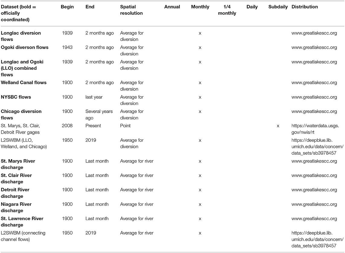
Table 2. Connecting channel and diversion flow products.
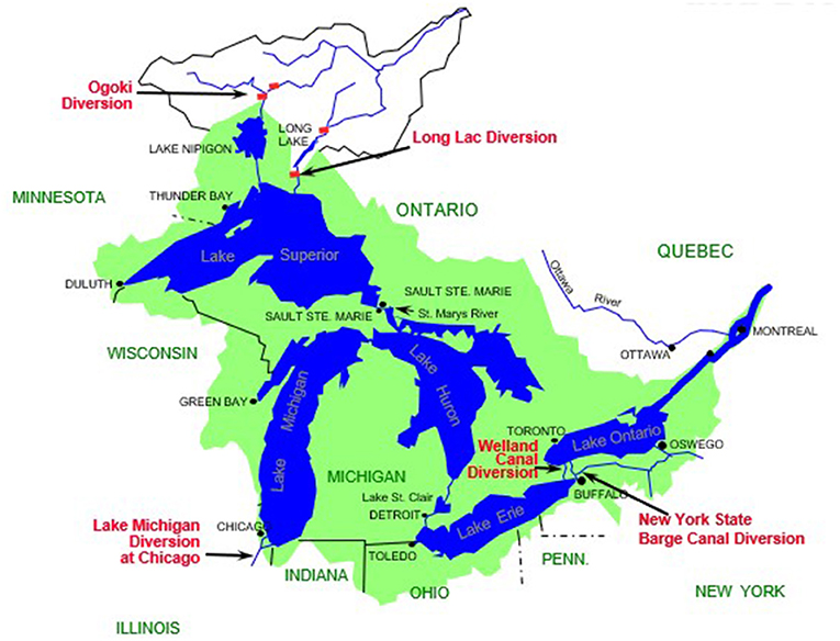
Figure 3. A view of the Great Lakes basin, highlighting the diversions in the system. Source: USACE, Detroit.
Long Lac and Ogoki
The Long Lac Diversion was completed in 1941 and flows into Lake Superior via the Aguasabon River with headwaters at the Kenogami River (International Joint Commission, 1985). The Ogoki Diversion was completed in 1943 and connects the Ogoki River to Lake Nipigon, which then flows into Lake Superior (International Joint Commission, 1985). Since they both flow into Lake Superior, they are usually referenced together as the Long Lac and Ogoki Diversions. Both diversions are located on the Canadian side of the border and are operated by Ontario Power Generation (OPG), which provides hydropower generation to northern Ontario. The combined diversion flow averages about 150 m3/s (5,300 ft3/s) into Lake Superior. Measured flows are made available by OPG and provided to ECCC for Great Lakes water budget monitoring efforts. Information on monthly flow rates derived from OPG reports can be obtained from the Coordinating Committee.
Chicago
The Chicago Diversion diverts water out of Lake Michigan. In 1900, the construction of the Chicago Sanitary and Ship Canal was completed and in 1922 the Calumet-Sag Channel was completed, which allowed the water to be diverted out of Lake Michigan into the Illinois River system (Figure 4; International Joint Commission, 1985). There are multiple components of the diversion, such as lockages, leakages, navigation make-up flow, and discretionary flow, which contribute to the total flow (Lake Michigan Diversion Committee, 2019). The total diversion flow is set by a Supreme Court Decree, which was last modified in 1980, that allows a total diversion of 91 m3/s or 3,200 ft3/s. The USACE Chicago District has the responsibility to monitor and audit the diversion. An annual report is published once a year that will contain the diversion accounting for one or more of the previous years. Data, reports, and further information can be found on the USACE Chicago District website at: https://www.lrc.usace.army.mil/Missions/Lake-Michigan-Diversion-Accounting/. Monthly flow rates derived from the USACE Chicago District reports can be obtained from the Coordinating Committee.
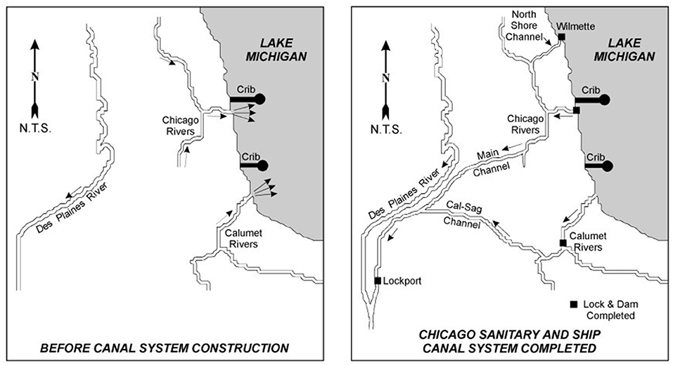
Figure 4. Before and after diagram of the Chicago diversion based on the completion of the canal system [source: United States Army Corps of Engineers (2019)].
Welland Canal
The Welland Canal was originally constructed in 1829, but has been modified and reconstructed and the current structure of the canal was completed in 1932 (International Joint Commission, 1985; St. Lawrence Seaway Management Corporation, 2003). The primary use for the canal was to provide a navigational route for ships that bypassed the Niagara Falls, however, the canal also provides water for hydropower, industrial and municipal uses. The present structure consists of eight locks that span between Port Colborne, Ontario and Port Weller, Ontario (St. Lawrence Seaway Management Corporation, 2003). The flow through the Welland Canal varies but is typically about 200 m3/s (7,100 ft3/s). The data is provided via the St. Lawrence Seaway Corporation. Monthly flow rates can be obtained from the Coordinating Committee.
New York State Barge Canal
The New York State Barge Canal takes water from the Niagara River at Tonawanda, NY and returns it back to Lake Ontario via tributaries and the Oswego Canal (International Joint Commission, 1985). The amount of water diverted varies by the time of year, but ultimately has no hydraulic effect on the Great Lakes. During the navigation season, the flow is estimated to be 31 m3/s (1,100 ft3/s) (International Joint Commission, 1985). Since 1956, the winter flow estimate is typically 0 m3/s due to the gates installed on the Erie Canal at Pendleton, which will close the canal for maintenance and repair. The New York State Barge Canal data is provided by the New York State Canal Corporation. Flows prior to 1951 are documented in reports (International Niagara Falls Engineering Board, 1953). Monthly flow rates can be obtained from the Coordinating Committee.
Connecting Channel Flows
Connecting channel flows are shown in Table 2. In the Great Lakes basin, the Great Lakes and Lake St. Clair are connected by the connecting channels, which are the St. Marys River, St. Clair River, Detroit River, Niagara River, and the St. Lawrence River.
St. Marys River
The amount of water that flows through the St. Marys River is prescribed monthly by the International Lake Superior Board of Control (ILSBC), although actual flow can differ from the prescribed flow due to potential unintentional deviations and differences between expected minor components (e.g., lockages and domestic use) and actual flows of these smaller components. The ILSBC was established by the International Joint Commission (IJC) through a 1914 Order of Approval (International Joint Commission, 1914), which gives the Board the objective to regulate the outflow from Lake Superior. There have been Supplementary Orders of Approval (https://ijc.org/en/lsbc/who/orders) over the years that have included updates to procedures and regulation plans that have been used to determine the flow. The current regulation plan is Plan 2012, which was implemented in January 2015 because of the 2014 Supplementary Order of Approval (International Joint Commission, 2014).
Plan 2012 provides operational guidelines and procedures to be followed when determining outflow each month. The main objective of Plan 2012 is to regulate outflow with consideration of conditions that are occurring both upstream and downstream, while maintaining much of the natural variability in lake levels. This is achieved by using a pre-project flow relationship, which is the flow that would have occurred prior to the canals and dams being built in the St. Marys River. This preproject relationship is based on the year 1887, which is generally thought of as the last year of the natural system (Clites and Quinn, 2003). Also, further adjustments are made by a balancing factor that adjusts flows depending on the level of Lake Superior and Lake Michigan-Huron relative to seasonal targets based on average conditions. Lastly, operational and physical limits are applied. Some examples of when limits would need to be considered include stable ice formation in the St. Marys River, conditions in regard to navigation or hydropower, flood risk, and safe operations of the control structures (International Lake Superior Board of Control., 2016). Once the total outflow for the month is determined, the flow is allocated through various control structures on the St. Marys River (Figure 5). This accounts for flow that is used for fish passage and other environmental considerations in the St. Marys Rapids, navigation and domestic users, and flow that goes to U.S. and Canadian hydropower plants (International Lake Superior Board of Control., 2016). For more information on the ILSBC, the current regulation plan, and flow data, visit the Board's website at https://www.ijc.org/en/lsbc.
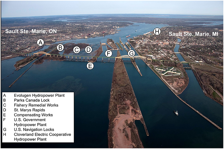
Figure 5. View of the various structures at the head of the St. Marys River that are considered in determining monthly outflow from Lake Superior (source: ILSBC).
As noted above, the actual flow through the St. Marys River can differ from the prescribed flow for unforeseen reasons. Therefore, the ILSBC determines the actual flow after-the-fact by summing the various components of flow through the structures in Figure 5 (referred to as “flow accounting”). These component flows are determined using reports from the various contributing agencies shown in Figure 5. These monthly flows can be obtained from the Coordinating Committee. In addition to the historical flows determined using flow accounting, real-time point estimates of discharge on the St. Marys River are available at U.S. Geological Survey (USGS) station 04127885. This station is operated through collaboration among USGS, ECCC, and USACE.
St. Clair River and Detroit River
Water flows out of Lake Huron and enters Lake St. Clair via the St. Clair River and then water leaves Lake St. Clair via the Detroit River into Lake Erie. The flows through the St. Clair River and Detroit River are unregulated and are coordinated periodically between federal agencies in the U.S. and Canada through the auspices of the Coordinating Committee. In the past, the flows have been calculated monthly using stage fall discharge (SFD) relationships and unsteady flow models. Reports produced by the committee have tracked these changes over time (Coordinating Committee on Great Lakes Basic Hydraulic Hydrologic Data, 1982, 1988; International Upper Great Lakes Study Board, 2009; Thompson et al., 2020). Most recently, index-velocity ratings have been used to calculate discharge measurements for the St. Clair River and Detroit River since 2009 (Thompson et al., 2020). The development of acoustic Doppler velocity meters (ADVMs) and index-velocity ratings has allowed for high temporal resolution computation and reporting of discharges. The method was developed by Levesque and Oberg (2012). ADVMs were installed in the St. Clair River at Port Huron and in the Detroit River at Fort Wayne in 2008 (Thompson et al., 2020) and since 2009 the daily data have been used to estimate the monthly average flow in the St. Clair and Detroit Rivers (McClerren, 2021). The data at these gages on the St. Clair at Port Huron and Detroit River at Fort Wayne are provided by USGS (stations 04159130 and 04165710). In the absence of data at these ADVM gages for more than a 24-h period, the SFD equations would be used to compute the flow by the Coordinating Committee (Thompson et al., 2020).
Niagara River
The outflow from Lake Erie into Lake Ontario is computed in two parts, first, the discharge in the Niagara River, and second, the discharge through the Welland Canal, although the discharge through the Welland Canal is typically <5% of the Niagara River discharge. The Niagara River section has many flow components shown in Figure 6.
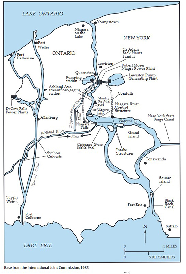
Figure 6. Map of the Niagara River and Welland Canal [source: Neff and Nicholas (2005)].
The Niagara River flow is determined by accounting for flows at different parts of the river, including the outflow from the Maid-of-the-Mist (MoM) Pool, diversion through the New York State Barge Canal, the flow over the Niagara Falls, Welland River flow, flow diverted to hydropower entities in U.S. and Canada, and locally estimated flows. The MoM outflow (QMoM) is determined using the rating equation shown in Equation (2).
In Equation (2), AA represents the water level at the Ashland Avenue gage (shown Figure 6) in meters.
Over time, this rating equation has been adjusted, due to changes in the river and gauging stations (Noorbakhsh, 2009). Each month, flows are estimated for the Niagara River at Buffalo (QBuffalo) by summing the outflow at the MoM Pool, flow diverted for hydropower, and the New York State Barge Canal Diversion, and subtracting local inflows and the portion of the Welland Canal Diversion (Welland River) that is returned to the river upstream of the Falls using Equation (3) (Noorbakhsh, 2009).
In Equation (3), BD is the water diverted to the Sir Adam Beck Power Plants, MD is the water diverted to the Robert Moses Niagara Power Plant, NYSBCD is the New York State Barge Canal Diversion flow, WR is the Welland River flow, and the LI is local inflows. This is also represented in Figure 7.
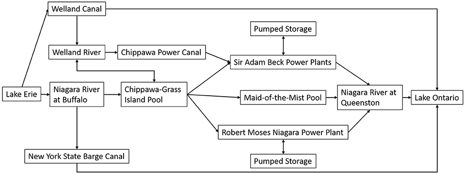
Figure 7. Diagram of how water flows from Lake Erie to Lake Ontario. Note that the size of the arrows does not reflect the relative size of the flows. For example, the arrow pointing from the Welland Canal to the Welland River represents a siphon system discharging only about 6 m3/s, compared to flows of around 8,000 m3/s for the Niagara River at Buffalo [adapted from: Coordinating Committee on Great Lakes Basic Hydraulic Hydrologic Data (1976)].
The MoM flow, Beck, and Moses discharges and diversions are provided by the International Niagara Committee, which includes the New York Power Authority and Ontario Power Generation. The Welland Canal River flow and Diversion flow are provided by the St. Lawrence Seaway Management Corporation (SLSMC). The New York State Barge Canal data is provided by the New York State Canal Corporation. Monthly Niagara River flows can be obtained from the Coordinating Committee.
St. Lawrence River
Water leaving Lake Ontario flows through the St. Lawrence River, which eventually leads to the Atlantic Ocean. Flow through the St. Lawrence River is primarily determined by the flow through the hydropower plants, which include the Moses-Saunders and Long Sault Dams. These computations are performed by the hydropower operators and the ratings are regularly verified by ECCC field staff using a vessel mounted acoustic Doppler current profiler. Discharges are reported to the International Lake Ontario-St. Lawrence River Board (ILOSLRB). However, other smaller components of the total flow also must be accounted for and this includes flow through the navigation canals and water diverted for domestic use. This Board of Control was established in 1952 under its first Order of Approval through the IJC (International Joint Commission, 1952). Outflows have been regulated since 1960, however, through Supplemental Orders of Approval modifications have been made to the regulation plan over time (International Joint Commission, 2016). The most recent Supplemental Order of 2016 commenced the Plan 2014 as the regulation plan to aide in determining outflows. The flow is primarily regulated through the Moses-Saunders Dam, which is located near Cornwall, ON and Massena, NY and jointly owned and operated by OPG and NYPA (International Lake Ontario St. Lawrence River Board, 2020).
Plan 2014 determines its weekly outflow based on the inflow of water to the lake from Lake Erie, water supplies to the lake via components (precipitation, runoff, and evaporation), the water level of Lake Ontario, and conditions upstream and downstream of the lake. Also, physical and operational limits are considered in regard to navigation and municipal uses, hydropower, flood risk, and stable ice formation in the St. Lawrence River in the winter.
For more information on the regulation, history, and flow data, visit https://ijc.org/en/loslrb and https://ijc.org/en/loslrb/watershed/outflow-changes. Monthly flows can also be obtained from the Coordinating Committee.
Net Basin Supply
From a lake water balance modeling perspective, it is convenient to combine over-lake precipitation, over-lake evaporation, and lateral tributary runoff into a single term representing the portion of a lake's water originating within a lake's basin (exclusive of connecting channel inflows and outflows). This single term is commonly referred to as a lake's net basin supply (or NBS).
There are two methods for estimating the NBS: the residual NBS (NBSR, computed from change in storage (dS), inflows (Qin), and outflows (Qout) using a water balance approach) and the component NBS (NBSC, computed as the sum of overlake precipitation (P), overlake evaporation (E), and lateral tributary runoff (R) into the lakes). The component and residual NBS are derived by rearranging the lake water balance (Equation 1), shown in Equations (4, 5).
In practice, the residual NBS is considered to be more easily observed, due to the challenges of estimating the overlake precipitation, evaporation, and lateral tributary runoff into the lakes resulting from vast ungaged areas over the lakes themselves and data discontinuities across the U.S.-Canada border. Net basin supply and its components are shown in Table 3.
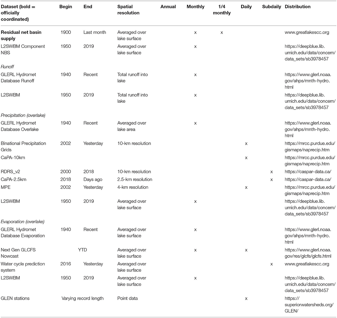
Table 3. Net basin supply (NBS) and NBS component data products.
Residual Net Basin Supply
The Coordinating Committee computes the residual NBS (in m3/s) using Equation (6):
where k is a conversion factor based on lake surface area.
Change in storage is calculated by taking the difference in water levels from the beginning to the end of a time period, typically monthly, that describes the total sum of water entering and leaving the lake via the components described above. Beginning of Month levels are determined using the approach described in Section Water Levels. Inflows and outflows are determined using diversion flows and connecting channel flows described in Sections Diversion Flows and Connecting Channel Flows. Note that the NYSBC diversion does not factor into any NBSR calculations, as water is diverted from the Niagara River and returned to Lake Ontario.
Residual NBS is another dataset that is coordinated by the Coordinating Committee, and coordinated data go back to 1900. The long historical record of this dataset makes it acceptable to be used in operational and regulation efforts that are conducted on both sides of the border (International Upper Great Lakes Study, 2012). However, there can be uncertainties when calculating NBS due to the magnitude of connecting channel flows and change in storage (Neff and Nicholas, 2005) in addition to other uncertainty in minor diversions, consumptive use, and thermal volumetric changes (Bruxer, 2010; International Upper Great Lakes Study, 2012). Despite uncertainties, this dataset helps water management agencies express water supply in the Great Lakes over an extended historical period and can provide insight moving forward in our changing climate.
Component Net Basin Supply and Lumped P, E, R Estimates
Component NBS
For decades, Great Lakes scientists had followed a practice of combining individual estimates of P, E, and R (sometimes from different data sources) to estimate NBS. However, even when these estimates come from a common model, we find that none of these models explicitly constrain them to be faithful to the water balance. Relatively recently, regional scientists developed a statistical model, commonly called the Large Lake Statistical Water Balance Model (L2SWBM) that assimilates output from multiple models and data sets to infer constrained estimates of each water balance component, for each lake, that is consistent with all other water balance components across the Great Lakes system (including observed changes in lake storage). As such, simulations from L2SWBM are generally considered to be the only source of component NBS that is faithful to the holistic water balance. For a recent data product produced by L2SWBM, see Do et al. (2020).
Precipitation
Although precipitation is also included in forcing datasets described in Section Meteorological Data, it is included here in order to specify datasets that can be used for representing the overlake component of net basin supply. As noted in the introduction, the challenge of representing this important NBS component is complicated by both the vast surface area of the lakes themselves, resulting in the need to interpolate surface observations over broad areas, as well as the international border, resulting in discontinuities in some datasets. As a result, a handful of Great Lakes specific datasets have been developed for the purpose of water supply monitoring and simulation (Table 3).
The GLERL Hydrometeorological Database overlake precipitation uses a Thiessen weighting approach to compute overlake precipitation [described by Hunter et al. (2015)]. This dataset is not an operational dataset, and is updated on a roughly annual basis for the purpose of providing data for research to monitor the Great Lakes water balance.
More recently, to support Coordinating Committee needs, the Midwest Regional Climate Center has operationalized a binational gridded precipitation product that combines the state-of-the-art operational precipitation products from the U.S. and Canada. The current version of this gridded bi-national product (referred to as “Binational Precipitation Grids” in Table 3) blends the 10-km Canadian Precipitation Analysis (CaPA, described by Fortin et al., 2015 and Lespinas et al., 2015) with the U.S. Multi-sensor Precipitation Estimate [MPE, described by Kitzmiller et al. (2013)] resampled to the same 10-km grid. These two products combine gage and radar data, and CaPA also includes a numerical weather prediction model. An archive of this binational gridded data and anomalies can be accessed through the Midwest Regional Climate Center. This product represents a promising pathway for developing future coordinated datasets produced by the Coordinating Committee. It is worth noting that as a result of the collaborative process of blending the two data sets, special attention has been given to improving the representation of precipitation by the two products over the lakes and across the border.
In addition to contributing to the binational gridded precipitation product, various versions of the CaPA product are available at multiple resolutions through the Canadian Surface Prediction Archive (CaSPAr). Among these CaPA products is the 10-km precipitation included in the Regional Deterministic Reanalysis System (v2), described in Section Reanalysis (referred to as RDRS_v2 in Table 3). The reanalysis includes hourly data from 1980–2018. It is anticipated that, due to the use of modeled data in addition to surface observations, estimates of historical overlake precipitation derived from this reanalysis product will be a more appropriate representation of actual overlake precipitation than the Thiessen-weighting product provided with the GLERL Hydrometeorological Database.
The other Great Lakes specific dataset comes from the L2SWBM via Do et al. (2020), described in Section Component NBS.
Runoff
The precipitation that falls on the land surface can take various paths to get to the lakes, this can be by overland flow across the land surface, sub-surface flow through the top soil layers, or baseflow through the groundwater system. The combination of these flows can be summed for each grid square or hydrological unit and is the more traditional definition of runoff for the scientific community; for example, when obtaining data from a reanalysis product such as the North American Land Data Assimilation System (NLDAS) or the European Centre for Medium-range Weather Forecasts (ECMWF) reanalyses.
The runoff from the land surface travels down the streamflow channels to eventually be deposited into the lakes. For the purposes of the calculation of NBS, the runoff for each lake is the amount of water that enters the lakes through the incoming river systems, with the exception of the flow from the upstream lake if there is one. Ideally, all of these rivers would have their flow measured at the point that they enter the lakes, however this is only true on a small number of the rivers in the Great Lakes. The percentage of the drainage area that is gaged varies depending on the lake and often the most downstream station may not be close to the outlet into the lake [for a representation of the portion of the basin that is gaged over time, see Fry et al. (2013)]. The location of gauging stations is often determined by local considerations and thus may not be the ideal location for the purpose of calculating flow into the lakes. Thus, there is a requirement to model the ungaged portion of the basin in some manner.
This modelling can range from simple area-ratio methods that transfer the amount of measured flow proportionally to the ungaged areas to sophisticated hydrological models that simulate the flow of water throughout the water cycle. The choice of model that is used can be based on many factors such as the final use of the results, the time required to run the model, or the availability of the input data. At the time of writing of this manuscript, there are two publicly available datasets for total runoff into the lakes. The GLERL Hydrometeorological Database (Hunter et al., 2015) includes runoff estimates computed using an area ratio estimate using a set of “most downstream” gages (Croley II and Hartman, 1986; Croley II and He, 2002). This approach has been shown to provide reliable estimates of total discharge to the lakes for gage combinations with similar catchment characteristics to the outlet's catchment (Fry et al., 2013). The second publicly available historical runoff dataset comes from the L2SWBM (described in Section Component NBS), and includes uncertainty estimates determined by resolving the Great Lakes water balance (Do et al., 2020).
There are many different agencies and research groups that run hydrological models around the Great Lakes, however there are only a few agencies that have an interest in obtaining data from both sides of the international border. Of course, flows from both sides of the international border are required in order to calculate the runoff into the lakes.
Initiated in 2014, the Great Lakes Runoff Intercomparison Projects (GRIP) are a series of studies that have focused on comparing the runoff generated by models from various academic institutions and federal agencies. The first study concentrated on Lake Michigan (Fry et al., 2014), second on Lake Ontario (Gaborit et al., 2017), and a third on Lake Erie (Mai et al., 2021a). The latest of the GRIP projects involves a wide range of lumped and distributed models that are being run over the entire Great Lakes watershed (Mai et al., 2021b), and represents an example of productive coordination between the research community and the Great Lakes water management community. In addition to including a broader variety of models, the later phases of GRIP have evolved to harmonize both the input datasets as well as the land surface database used by all models for both calibration and verification. It is hoped that once this latest GRIP project is completed, at least some of the different models would be adopted for operational monitoring of runoff by the Great Lakes water management community.
Evaporation
Like most runoff estimates, evaporation estimates for the Great Lakes are primarily determined using models driven by atmospheric forcing. There are a number of models that have been developed and applied specifically to the Great Lakes for simulating total evaporation from the lakes' surfaces. The GLERL Hydrometeorological Database, for example, provides time series of monthly evaporation from each of the lakes, computed by the Large Lake Thermodynamics Model [LLTM, described by Croley II (1989)]. The LLTM is a 1-dimensional thermodynamics model that computes evaporation by simulating the energy balance in the atmosphere above the lake, heat storage throughout the lake's vertical column, and aerodynamic evaporation. The estimates provided in the GLERL Hydrometeorological Database are driven by meteorological forcing computed by interpolation of surface observations using a Thiessen weighting approach. More recently, GLERL has begun providing estimates of lake-wide average evaporation aggregated from output from Next Generation Great Lakes Coastal Forecast System nowcast (Anderson et al., 2018). Fluxes in the Next Generation GLCFS are computed by experimental runs of the Finite Volume Coastal Ocean Model (Chen et al., 2003).
Atmospheric reanalyses and General Circulation Models (GCMs) also provide estimates of over-lake evaporation, however, the representation of lakes within the modeling system can considerably alter the simulation of lake-effect processes and lake-atmosphere interactions. In such modeling systems, lakes are either represented by prescribing the lake surface water temperatures through various observational and operational sources or parameterized through shallow 1-dimensional lake models, while inclusion of more involved 3-dimensional lake models is generally absent in Earth System Models due to computational costs and other challenges (Mironov et al., 2010; Fiedler et al., 2014; Minallah and Steiner, 2021b,c). It is important to note that differences in lake representation in models can considerably alter the lake surface water temperatures, evaporation, and lake-effect precipitation magnitudes. For example, Minallah and Steiner (2021c) assess the effects of lake representation differences between two generations of the ECMWF reanalyses, ERA-Interim and the newer ERA5, where the former prescribes surface temperatures through external data sources while the later introduces the 1-dimensional Freshwater Lake (FLake) model. This difference in lake simulation resulted in ERA5 showing much warmer Great Lakes surface temperatures (by up to 5K) in the summer and producing twice the magnitude of evaporation as compared to ERA-Interim. This significantly alters the simulation of the regional hydroclimate and the water cycle both on climatological and short-term meteorological timescales between these two datasets, emphasizing the importance of careful examination of how lakes are simulated in the models before conducting more involved regional hydroclimatic assessments.
Validation of simulated evaporation by models can be a challenge due to spatial sparsity of buoy data and general absence of spatiotemporally consistent observational datasets. The Great Lakes Evaporation Network (GLEN) currently provides flux tower observations of evaporation for six sites over the Great Lakes, with four platforms located on offshore lighthouse sites (Stannard Rock, White Shoal, Spectacle Reef, shown in Figure 8, as well as Granite Island located on Lake Superior) and the remaining two located on nearby land. Half hourly data for each station are available, which have undergone only basic flux corrections, so careful pre-processing is required before it can be used to validate model outputs. The GLEN station data has been used to assess and improve Great Lakes hydrodynamics models (e.g., Durnford et al., 2018; Fujisaki-Manome et al., 2020). However, similar analyses have not been conducted between the lake surface fluxes from earth systems models and these stations. A visual comparison is included here in Figure 8, and indicates that both the global products and station data likely have significant biases that would need to be corrected before application to Great Lakes regional climate studies and water resources management.
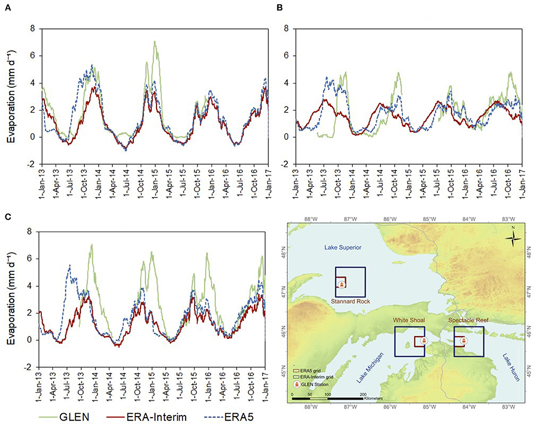
Figure 8. 30-day running mean evaporation rate (mm/day) for three GLEN stations (location shown on map) and corresponding magnitudes for ERA-Interim (0.75°) and ERA5 (0.25°) grid cells. The running mean is computed after pre-processing and removal of erroneous and extreme values in the GLEN station data. (A) Stannard rock. (B) White Shoal. (C) Spectacle Reef.
Lake Surface Water Temperature (LSWT) and Ice Cover
Lake surface water temperature (LSWT, shown in Table 4) is one of the primary drivers of the lake-atmosphere interaction and related processes; e.g., lake-effect precipitation, lake breeze circulation patterns, cloud formation, etc. (Wright et al., 2013; Laird et al., 2017; Minallah and Steiner, 2021c). These LSWT are highly sensitive to climate warming and show an amplified response as compared to the surrounding land (Zhong et al., 2016; Kravtsov et al., 2018). Recent research has shown that LSWT have increased worldwide along with air temperatures, which has implications for ecosystems and water supply (Woolway et al., 2020). Further, the Coupled Model Intercomparison Project (CMIP) 6 projections reveal that earth systems models with some lake representation simulate a higher increase in the lake surface evaporation as compared to the surrounding land by the mid-century, especially in the winter months (Minallah and Steiner, 2021b) which has implications for NBS assessments. Interestingly, there is far less monitoring of subsurface temperatures, although the subsurface observations can provide indication of changes in thermal regimes in the lakes (Anderson et al., 2021).
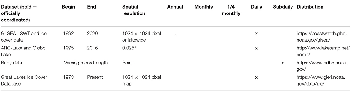
Table 4. Lake surface water temperature (LSWT) and ice cover data products.
LSWT can be measured both directly over the water body (buoy data) and through satellite retrievals of the water surface temperature. For the Great Lakes, two main satellite-derived LSWT datasets are available. The first is the Great Lakes Surface Environmental Analysis (GLSEA) Surface Water Temperature, produced by NOAA Great Lakes Environmental Research Laboratory using AVHRR (Advanced Very High Resolution Radiometer) imagery from the NOAA satellite series. This data is available for the 1992–2020 period as 1024 × 1024 pixel maps or as lake-averaged temperatures. The second dataset is produced at the University of Reading using the Earth Observing missions of the European Space Agency for all lakes globally (including lakes in the Great Lakes basin). This includes the ARCLake (Along-Track Scanning Radiometer (ATSR) Reprocessing for Climate: Lake Surface Water Temperature and Ice Cover) dataset and the newer generation GloboLakes (Global Observatory of Lake Responses to Environmental Change) dataset. Both datasets provide daily LSWT averages, with the GloboLakes having a finer resolution of 0.025 × 0.025 (1995–2016 period), while ARCLake has a resolution of 0.05 × 0.05 (1995–2013 period; Merchant and MacCallum, 2018; Carrea and Merchant, 2019).
While these datasets provide high resolution estimates of LSWT, caution must be exercised in their use as satellite retrievals can have errors due to sensor limitations, especially under cloudy conditions. Past assessment of these datasets for the Great Lakes region (Minallah and Steiner, 2021c) has shown spatiotemporal inconsistencies in data availability that introduce biases in lake-averaged measurements. This issue is especially pronounced in the winter months when data availability is almost non-existent and lake averages produce relatively warmer LWSTs. For example, Figure 9B shows the long-term lake-average LSWT for the three satellite-based datasets and different reanalyses over Lake Superior, where the months from Jan to Mar are consistently warm (~275 K) for the three satellite-based datasets, whereas the reanalysis datasets show varying magnitudes below 273 K, depending on how lakes are simulated in these models. For GLSEA, we again note that while there is a clear distinction in the LSWT for the five Great Lakes in the summer months (with Lake Erie being the warmest and Lake Superior coldest), the winter months show near same magnitude of ~275 K for all the lakes (Figure 9A).
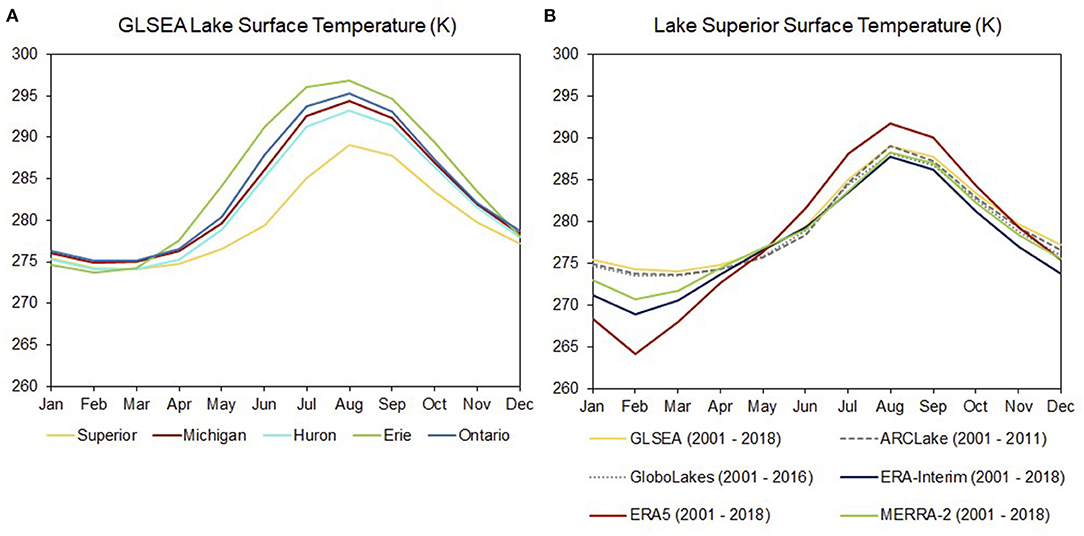
Figure 9. 2001–2018 climatology of lake-average GLSEA LSWT for the five Laurentian Great Lakes (A) and Lake Superior LSWT for the different satellite-based and reanalysis datasets [(B); averaging period included in the legend]. (B) Is adapted from Minallah and Steiner (2021c).
For the summer months (ice-free season), buoy observations for the lake surface and air temperatures are also available; however, buoys are removed at the end of the autumn season and therefore they cannot supplement the satellite-derived LSWT for winter months to establish the ground truth (Gronewold and Stow, 2014).
In addition to LSWT, surface ice cover data (also shown in Table 4) is informative for verification of lake thermodynamics models. NOAA Great Lakes Environmental Research Laboratory maintains a Great Lakes Ice Cover Database, which compiles data from the Great Lakes Ice Atlas [1973–2002, described by Assel et al. (2002)], with addendums in separate reports for 2003–2005 described by Assel (2005) and updates for 2006-present using the same methods as the Great Lakes Ice Atlas (Wang et al., 2012, 2017). Daily gridded data are available for the ice season, which varies somewhat by year.
Meteorological Data
Global and regional meteorological data products, including precipitation, are included in Table 5.
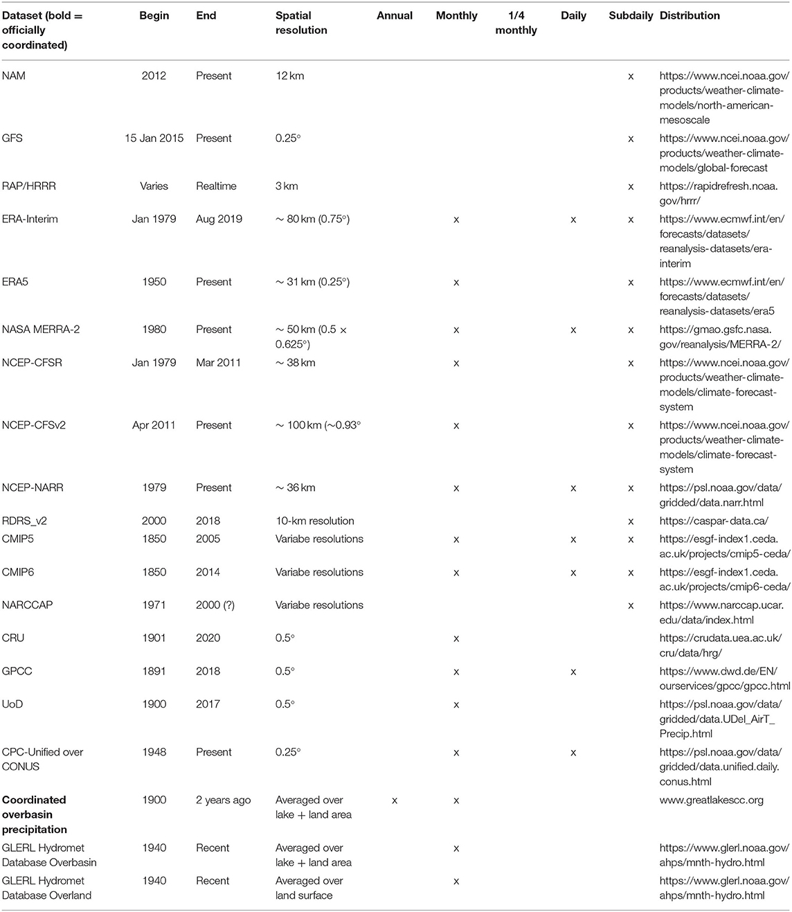
Table 5. Meteorological forcing data products.
Precipitation
Various global-scale observation-based gridded precipitation products are available for assessment of precipitation time series and spatial patterns; however, due to lack of observations over the lake surfaces and employment of land-based gage measurements, these products are better suited for over-land analyses. Commonly used global datasets include CRU time series (University of East Anglia Climate Research Unit; Harris et al., 2014), UoD time series (University of Delaware Global Land Data; Willmott, 2000), GPCC dataset (Global Precipitation Climatology Center; Schneider et al., 2014), and NOAA CPC Unified Gauge-Based Analysis over CONUS. These datasets can provide an adequate benchmark for assessment of model outputs (Figure 10); however, the quality of the time series is affected by the varying gage density both spatially and temporally. In general, their time series are similar in magnitudes, however, we note some differences from 1997 onward, likely due to differences in the number of gages assimilated to produce the gridded products.
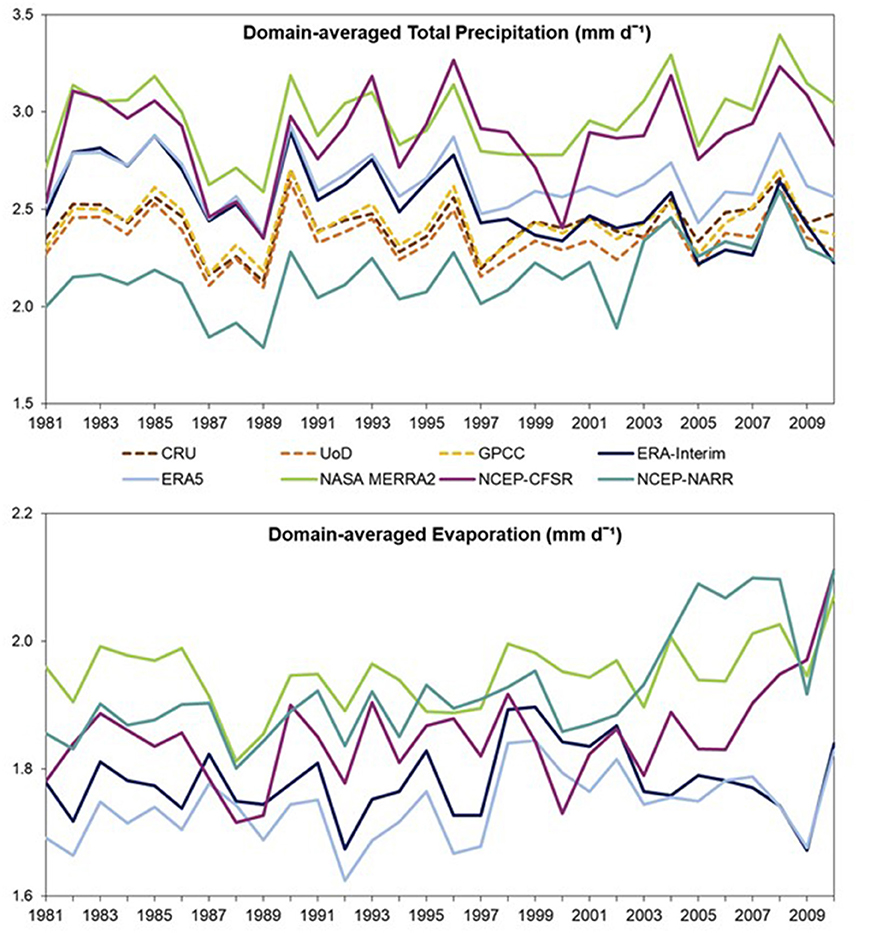
Figure 10. Great Lakes domain-averaged (40–51 N, 74–94 W) precipitation and evaporation timeseries as simulated by various reanalysis datasets. Dashed lines in the top panel show gridded gage-based precipitation products.
In addition to the gridded products described above, several precipitation products have been developed specifically for the Great Lakes region. For example, the Coordinating Committee produces monthly overbasin (including lake and land area) precipitation estimates on an annual basis. A primary goal of the coordinated dataset is to provide a long term record of precipitation that can be used to compute anomalies and statistics in order to monitor the water budget of the Great Lakes. Accordingly, the coordinated precipitation product is compiled from a number of interpolated station-based datasets with records dating back to 1900. At the time of writing of this manuscript, the coordinated dataset includes data from three interpolated products: the U.S. Army Corps of Engineers' Areally-Weighted District product (1900–1930), the NOAA GLERL Monthly Thiessen Polygon estimates (1931–1947), and daily Thiessen polygon estimates produced by the Great Lakes Seasonal Hydrologic Forecasting System (referred to as GLSHyFS, 1948-recent). These three products are described by Hunter et al. (2015), however it should be noted that the GLSHyFS software has replaced the Great Lakes Advanced Hydrologic Prediction System which was previously used to compute the daily estimates, and recent quality control efforts have resulted in using a smaller set of station observations. The GLERL Hydrometeorological Database also includes GLSHyFS-derived estimates of precipitation, which also include overbasin and overland precipitation in addition to the overlake precipitation described in Precipitation. These lumped estimates are conventionally used to (a) develop climatologies and (b) drive lumped rainfall-runoff models, notably the Large Basin Runoff Model, which is used to inform the U.S. contribution to the internationally coordinated 6-month Great Lakes water level forecast (Fry et al., 2020). In addition, the binational precipitation grids and CaPA products described in Section Precipitation are consistent across the border.
Reanalysis
Reanalysis products are helpful to provide a consistent process-based assessment of the various hydroclimatic variables and can be used as both forcing or validation datasets for hydrological modeling. Due to limitations of the interpolated gage-based estimates, reanalysis datasets are often more suitable and accurate (Essou et al., 2017). The commonly used global reanalyses are listed in Table 5. Past assessments on inter-comparison of these datasets reveal that the regional reanalysis NCEP-NARR has lowest overall magnitudes of precipitation but one of the highest magnitudes for evaporation (Figure 10), especially in the summer months. The other NCEP product, Climate Forecast System Reanalysis (CFSR), has considerable biases in the seasonal cycle of precipitation and evaporation, despite getting relatively reasonable estimates of the annual magnitudes. These reanalyses are somewhat inadequate in capturing the various water budget quantities. NASA MERRA-2 reanalysis is also relatively wetter as compared to gage-based datasets and other reanalyses (Figure 10) and is especially wet in the spring and early summer months (Minallah and Steiner, 2021a). The two ECMWF reanalyses (ERA-Interim and ERA5) generally capture better annual and seasonal magnitudes; however, as explained in Section Evaporation, the differences in how lakes are simulated in the two versions result in significant differences in the over-lake conditions which subsequently alters the simulation of lake-effect processes. Therefore, users must exercise caution in employing these datasets as their quality will depend on the spatiotemporal scales and objectives of the study.
In addition to the global products described above, one newer surface reanalysis product that is noted to be of particular interest for transboundary and northern watersheds in North America is the Canadian 10 km North American precipitation and land-surface reanalysis (Gasset et al., 2021). This reanalysis (listed as RDRS_v2 in Table 5) is the result of initializing the Global Deterministic Reforecast System with ERA-Interim and dynamically downscaling the output using the Regional Deterministic Reforecast System (RDRS), coupled with the Canadian Land Data Assimilation System (CaLDAS) and the Canadian Precipitation Analysis (CaPA). The reanalysis includes hourly data from 1980 to 2018. Data are available for download from the Canadian Surface Prediction Archive (CaSPAr, at https://caspar-data.ca/). This product was used to construct the forcing for the later phases of the Great Lakes Runoff Intercomparison Project, described in Section Runoff.
High-Resolution Meteorological Forcing
Various numerical weather prediction model outputs are available as atmospheric forcing datasets for hydrological modeling. These include HRRR (High-Resolution Rapid Refresh), RAP (Rapid Refresh), GFS (Global Forecast System), and NAM (North American Mesoscale Forecast System). These operational datasets provide high resolution weather forecasts that are available on 3–6 hourly time steps for historical periods (2010's - present), but they do not go farther back in time. Furthermore, frequent changes in the model physics and assimilation schemes of the operational systems can introduce some irregularities if assessments over multiple years are conducted.
General Circulation Models (GCMs)
GCM outputs are often used as direct input to hydrological models as they can provide both historical simulations and future projections under various climate scenarios. Before conducting assessments of future changes in the hydrological cycle, assessment of historical simulation must be conducted as GCMs contain multiple biases, especially for precipitation (Sperna Weiland et al., 2010). For the Great Lakes region, such assessments have been conducted for GCMs participating in the CMIP5 and CMIP6 programs. Briley et al. (2021) conducted a usability study for CMIP5 climate models in the Great Lakes region and found that many GCMs do not simulate these lakes in a way that can capture their impact on the regional climate, therefore use of these models for future assessments is impractical. They propose a framework to categorize various CMIP5 GCMs under three categories; simulation of lake dynamics, crude representation of lakes, and absence of lake simulation. They concluded that only 4 CMIP5 GCMs have adequate representation of the lakes that provide credible information for practitioners.
For the most recent CMIP6, Minallah and Steiner (2021c) conducted an assessment of the water cycle as simulated by 15 available GCMs. They find that most GCMs (10/15) either do not simulate large inland water bodies at all (represented as land cells) or have major inconsistencies in how the lakes are simulated. They find that these lakes have prominent effects on moisture generation and distribution processes at both meteorological and climatic time scales. Therefore, representation of detailed lake processes in GCMs is important for accurate assessments of the regional hydroclimate. Dynamical downscaling of GCMs using regional climate models (RCMs) has emerged as an approach for improving the representation of lakes [see Delaney and Milner (2019) for a summary of recent developments in regional climate modeling for the Great Lakes]. Further, the GCMs that can provide credible information for hydrological modelers require bias-correction of the atmospheric variables (specifically precipitation) using the various station-based or reanalysis datasets before they can be input as forcing for hydrological models to ensure consistencies in surface runoff and streamflows.
Concluding Remarks
In conducting this exercise of aggregating and describing data sources for use in Great Lakes hydroclimate monitoring and simulation, we identified two key gaps that create barriers to appropriate data selection and application.
First, there are important successes in coordinating data for water management across the lakes and across the border; however, we find a general lack of shared documentation, communication, and data use across perspectives (i.e., water management and earth systems modeling communities). For many of the Great Lakes region specific datasets, there is a lack of formal documentation, or, where documentation does exist, it is in the form of reports (and sometimes internal operating procedures) that are not discovered under traditional academic research. On the other hand, important advancements achieved by the earth systems modeling community are not always evaluated, documented, or communicated with region-specific water management activities in mind.
Second, we find that this lack of formal documentation and communication results in earth system and forecast models being developed in the absence of consistent data across the U.S.-Canada border. If regional datasets are not consistent or readily available (in terms of format, accessibility, and discoverability), they will not be assimilated into earth systems models. Discontinuities across the border in region- or country-specific datasets often render them impractical for transboundary basin-wide assessments resulting in use of coarser and less precise, but spatiotemporally consistent, global datasets by the earth sciences community.
We make two recommendations to address the gaps identified above. First, we believe it is incumbent on the earth systems modeling community to engage regional practitioners to understand unique data gaps, limitations, and challenges, particularly those associated with monitoring and modeling large freshwater surfaces and domains that interact across an international border. Second it is imperative that the individuals and organizations that make up the water management community improve documentation and communication of region-specific hydroclimate data. This action will enable the global earth science community (and other research groups outside of the Great Lakes basin) to use the data that have been evaluated and coordinated across both sides of the international border. This advancement has the potential to broadly diversify the range of models and datasets available for improved understanding and management of water resources of the Great Lakes.
Author Contributions
LF led the development of the manuscript. LF, AG, FS, SM, and DA contributed sections of the manuscript. JF provided details on water level, connecting channel, diversion data products, and reviewed the manuscript. All authors contributed to manuscript revision, read, and approved the submitted version.
Conflict of Interest
The authors declare that the research was conducted in the absence of any commercial or financial relationships that could be construed as a potential conflict of interest.
Publisher's Note
All claims expressed in this article are solely those of the authors and do not necessarily represent those of their affiliated organizations, or those of the publisher, the editors and the reviewers. Any product that may be evaluated in this article, or claim that may be made by its manufacturer, is not guaranteed or endorsed by the publisher.
Acknowledgments
The authors gratefully acknowledge input and feedback during the development of the manuscript from Tim Calappi, Chuck Sidick, Matt McClerren, and Allison Steiner. In addition, we thank members and associates of the Coordinating Committee for their thoughtful review. This is NOAA GLERL contribution number 1998.
Supplementary Material
The Supplementary Material for this article can be found online at: https://www.frontiersin.org/articles/10.3389/frwa.2022.803869/full#supplementary-material
References
Anderson, E. J., Fujisaki-Manome, A., Kessler, J., Lang, G. A., Chu, P. Y., Kelley, J. G., et al. (2018). Ice forecasting in the next-generation great lakes operational forecast system (GLOFS). J. Mar. Sci. Eng. 6:123. doi: 10.3390/jmse6040123
Anderson, E. J., Stow, C. A., Gronewold, A. D., Mason, L. A., McCormick, M. J., Qian, S. S., et al. (2021). Seasonal overturn and stratification changes drive deep-water warming in one of Earth's largest lakes. Nat. Commun. 12, 1–9. doi: 10.1038/s41467-021-21971-1
Assel, R. A. (2005). Great Lakes Ice Cover Climatology Update, Winters 2003, 2004, and 2005. NOAA Technical Memorandum GLERL-135. Ann Arbor, MI: National Oceanic and Atmospheric Administration Great Lakes Environmental Research Laboratory.
Assel, R. A., Norton, D. C., and Cronk, K. C. (2002). A Great Lakes Ice Cover Digital Data Set for Winters 1973–2000. NOAA Technical Memorandum GLERL-121. Ann Arbor, MI: National Oceanic and Atmospheric Administration Great Lakes Environmental Research Laboratory.
Briley, L. J., Rood, R. B., and Notaro, M. (2021). Large lakes in climate models: a Great Lakes case study on the usability of CMIP5. J. Great Lakes Res. 47, 405–418. doi: 10.1016/j.jglr.2021.01.010
Bruxer, J. (2010). Uncertainty Analysis of Lake Erie Net Basin Supplies as Computed Using the Residual Method. (Master's thesis), McMaster University, Hamilton, ON, Canada.
Carrea, L., and Merchant, C. J. (2019). GloboLakes: Lake Surface Water Temperature (LSWT) v4.0 (1995–2016). Centre for Environmental Data Analysis, 29 March 2019. doi: 10.5285/76a29c5b55204b66a40308fc2ba9cdb3
Chen, C., Liu, H., and Beardsley, R. C. (2003). An unstructured grid, finite-volume, three-dimensional, primitive equations ocean model: application to coastal ocean and estuaries. J. Atmos. Oceanic Technol. 20, 159–186. doi: 10.1175/1520-0426(2003)020<0159:AUGFVT>2.0.CO
Clites, A. H., and Quinn, F. H. (2003). The history of Lake Superior regulation: implications for the future. J. Great Lakes Res. 29, 157–171. doi: 10.1016/S0380-1330(03)70424-9
Coordinating Committee on Great Lakes Basic Hydraulic Hydrologic Data (1976). Lake Erie Outflow 1860-1964 (with Addendum 1965-1975). Available online at: http://www.GreatLakesCC.org (accessed January 20, 2022).
Coordinating Committee on Great Lakes Basic Hydraulic Hydrologic Data (1982). Lakes Michigan–Huron Outflows, St. Clair and Detroit Rivers 1900–1978. Available online at: http://www.GreatLakesCC.org (accessed January 20, 2022).
Coordinating Committee on Great Lakes Basic Hydraulic Hydrologic Data (1988). Lakes Michigan–Huron Outflows, St. Clair and Detroit Rivers 1900–1986. Available online at: http://www.GreatLakesCC.org (accessed January 20, 2022).
Coordinating Committee on Great Lakes Basic Hydraulic Hydrologic Data (1992). IGLD 1985. Available online at: https://www.lre.usace.army.mil/Portals/69/docs/GreatLakesInfo/docs/IGLD/BrochureOnTheInternationalGreatLakesDatum1985.pdf (accessed January 21, 2022).
Coordinating Committee on Great Lakes Basic Hydraulic Hydrologic Data (2017). Updating the International Great Lakes Datum. Available online at: http://www.GreatLakesCC.org (accessed January 20, 2022).
Croley II, T. E. (1983). Great Lake basins (USA-Canada) runoff modeling. J. Hydrol. 64, 135–158. doi: 10.1016/0022-1694(83)90065-3
Croley II, T. E. (1989). Verifiable evaporation modeling on the laurentian Great Lakes. Water Resour. Res. 25, 781–792. doi: 10.1029/WR025i005p00781
Croley II, T. E., and Hartman, H. C. (1986). Near-Real-Time Forecasting of Large-Lake Water Supplies: A User's Manual. Ann Arbor, MI: NOAA Technical Memorandum ERL GLERL-61, Great Lakes Environmental Reesearch Laboratory. Available online at: https://www.glerl.noaa.gov/ftp/publications/tech_reports/glerl-061/tm-061.pdf
Croley II, T. E., and He, C. (2002). “Great Lakes large basin runoff model,” in Proceedings, Second Federal Interagency Hydrologic Conference. Las Vegas, NV.
Delaney, F., and Milner, G. (2019). “The state of climate modeling,” in The Great Lakes Basin – A Synthesis in Support of a Workshop Held on June 27, 2019 in Ann Arbor, MI (Toronto, CA: Ontario Climate Consortium), 1–80. Available online at: https://climateconnections.ca/app/uploads/2020/05/The-State-of-Climate-Modeling-in-the-Great-Lakes-Basin_Sept132019.pdf (assessed September 13, 2019).
Do, H. X., Smith, J. P., Fry, L. M, and Gronewold, A. D. (2020). Seventy-year long record of monthly water balance estimates for Earth's largest lake system. Sci. Data 7:276. doi: 10.1038/s41597-020-00613-z
Durnford, D., Fortin, V., Smith, G., Archambault, B., Deacu, D., Dupont, F., et al. (2018). Toward an operational water cycle prediction system for the Great Lakes and St. Lawrence River. Bull. Am. Meteorol. Soc. 99, 521–546. doi: 10.1175/BAMS-D-16-0155.1
Essou, G. R., Brissette, F., and Lucas-Picher, P. (2017). The use of reanalyses and gridded observations as weather input data for a hydrological model: comparison of performances of simulated river flows based on the density of weather stations. J. Hydrometeorol. 18, 497–513. doi: 10.1175/JHM-D-16-0088.1
Fiedler, E. K., Martin, M. J., and Roberts-Jones, J. (2014). An operational analysis of lake surface water temperature. Tellus A Dyn. Meteorol. Oceanogr. 66, 21247. doi: 10.3402/tellusa.v66.21247
Fortin, V., Roy, G., Donaldson, N., and Mahidjiba, A. (2015). Assimilation of radar quantitative precipitation estimations in the Canadian Precipitation Analysis (CaPA). J. Hydrol. 531, 296–307. doi: 10.1016/j.jhydrol.2015.08.003
Fry, L., Hunter, T., Phanikumar, M., Fortin, V., and Gronewold, A. (2013). Identifying streamgage networks for maximizing the effectiveness of regional water balance modeling. Water Resour. Res. 49, 2689–2700. doi: 10.1002/wrcr.20233
Fry, L. M., Apps, D., and Gronewold, A. D. (2020). Operational seasonal water supply and water level forecasting for the laurentian great lakes. J. Water Resour. Plan. Manag. 146:04020072. doi: 10.1061/(ASCE)WR.1943-5452.0001214
Fry, L. M., Gronewold, A. D., Fortin, V., Buan, S., Clites, A. H., Luukkonen, C., et al. (2014). The great lakes runoff intercomparison project phase 1: lake Michigan (GRIP-M). J. Hydrol. 519, 3448–3465. doi: 10.1016/j.jhydrol.2014.07.021
Fujisaki-Manome, A., Mann, G. E., Anderson, E. J., Chu, P. Y., Fitzpatrick, L. E., Benjamin, S. G., et al. (2020). Improvements to lake-effect snow forecasts using a one-way air–lake model coupling approach. J. Hydrometeorol. 21, 2813–2828. doi: 10.1175/JHM-D-20-0079.1
Gaborit, É., Fortin, V., Tolson, B., Fry, L., Hunter, T., and Gronewold, A. D. (2017). Great Lakes Runoff Inter-comparison Project, phase 2: lake Ontario (GRIP-O). J. Great Lakes Res. 43, 217–227. doi: 10.1016/j.jglr.2016.10.004
Gasset, N., Fortin, F., Dimitrijevic, M., Carrera, M., Bilodeau, B., Muncaster, R., et al. (2021). A 10 km North American precipitation and land-surface reanalysis based on the GEM atmospheric model. Hydrol. Earth Syst. Sci. 25, 4917–4945. doi: 10.5194/hess-25-4917-2021
Gronewold, A. D., Fortin, V., Caldwell, R., and Noel, J. (2018). Resolving hydrometeorological data discontinuities along an international border. Bull. Am. Meteorol. Soc. 99, 899–910. doi: 10.1175/BAMS-D-16-0060.1
Gronewold, A. D., and Rood, R. B. (2019). Recent water level changes across Earth's largest lake system and implications for future variability. J. Great Lakes Res. 45, 1–3. doi: 10.1016/j.jglr.2018.10.012
Gronewold, A. D., and Stow, C. A. (2014). Water loss from the Great Lakes. Science 343, 1084–1085. doi: 10.1126/science.1249978
Harris, I., Jones, P. D., Osborn, T. J., and Lister, D. H. (2014). Updated high-resolution grids of monthly climatic observations–the CRU TS3. 10 dataset. Int. J. Climatol. 34, 623–642. doi: 10.1002/joc.3711
Hunter, T. S., Clites, A. H., Campbell, K. B., and Gronewold, A. D. (2015). Development and application of a North American Great Lakes hydrometeorological database—part I: precipitation, evaporation, runoff, and air temperature. J. Great Lakes Res. 41, 65–77. doi: 10.1016/j.jglr.2014.12.006
International Joint Commission (1914). Orders of Approval. Available online at: https://ijc.org/sites/default/files/1914%20Order%20of%20Approval.pdf (accessed September 30, 2021).
International Joint Commission (1952). Hydro-Power – St. Lawrence River. Available online at: https://ijc.org/en/68a (accessed September 30, 2021).
International Joint Commission (1985). Great Lakes Diversions and Consumptive Uses: A Report to the Governments of the United States and Canada under the 1977 Reference. International Joint Commission. Available online at: https://www.ijc.org/sites/default/files/ID279.pdf (accessed October 26, 2021).
International Joint Commission (2014). Supplementary Orders of Approval. Available online at: https://ijc.org/sites/default/files/2014%20Supplementary%20Order%20of%20Approval.pdf (accessed September 30, 2021).
International Joint Commission (2016). Supplementary Orders of Approval. Available online at: https://ijc.org/sites/default/files/Docket_68_Order_Sup-RegulationOfLakeOntarioOutlfows-2016-12-08.pdf (accessed September 30, 2021).
International Lake Ontario St. Lawrence River Board (2020). Lake Ontario St. Lawrence River Regulation. Available online at: https://ijc.org/en/loslrb/who/regulation (accessed September 1, 2021).
International Lake Superior Board of Control. (2016). Operational Guide for Plan 2012. A Report to the International Joint Commission by the International Lake Superior Board of Control.
International Niagara Falls Engineering Board (1953). Preservation and enhancement of Niagara Falls, report to the International Joint Commission. Also included as part of report of the International Joint Commission of the same title. Washington, DC; Ottawa ON: International Niagara Falls Engineering Board.
International Upper Great Lakes Study (2012). Lake Superior Regulation: Addressing Uncertainty in Upper Great Lakes Water Levels. Available online at: https://legacyfiles.ijc.org/publications/Lake_Superior_Regulation_Full_Report.pdf (accessed October 15, 2021).
International Upper Great Lakes Study Board (2009). Impacts on Upper Great Lakes Water Levels, St. Clair River Final Report to the International Joint Commission. Available online at: http://www.iugls.org/Final_Reports (Accessed September 1, 2021).
Kitzmiller, D., Miller, D., Fulton, R., and Ding, F. (2013). Radar and multisensor precipitation estimation techniques in National Weather Service hydrologic operations. J. Hydrol. Eng. 18, 133–142. doi: 10.1061/(ASCE)HE.1943-5584.0000523
Kravtsov, S., Sugiyama, N., and Roebber, P. (2018). “Role of nonlinear dynamics in accelerated warming of great lakes,” in Advances in Nonlinear Geosciences, ed A. A. Tsonis (Berlin: Springer), 279–295. doi: 10.1007/978-3-319-58895-7_15
Laird, N. F., Metz, N. D., Gaudet, L., Grasmick, C., Higgins, L., Loeser, C., et al. (2017). Climatology of cold season lake-effect cloud bands for the North American Great Lakes. Int. J. Climatol. 37, 2111–2121. doi: 10.1002/joc.4838
Lake Michigan Diversion Committee (2019). Findings of the Eighth Technical Committee for Review of Diversion Flow Measurements and Accounting Procedures. Chicago, IL: United States Army Corps of Engineers.
Lakshmi, V., Fayne, J., and Bolten, J. (2018). A comparative study of available water in the major river basins of the world. J. Hydrol. 567, 510–532. doi: 10.1016/j.jhydrol.2018.10.038
Lemarquand, D. (1993). The International Joint Commission and changing Canada–United States boundary relations. Nat. Resour. J. 33, 59–91.
Lespinas, F., Fortin, V., Roy, G., Rasumussen, P., and Stadnyk, T. (2015). Performance evaluation of the canadian precipitation analysis (CaPA). J. Hydrometeorol. 16, 2045–2064. doi: 10.1175/JHM-D-14-0191.1
Levesque, V. A., and Oberg, K. A. (2012). Computing Discharge Using the Index Velocity Method. Reston, VA: US Department of the Interior, US Geological Survey. doi: 10.3133/tm3A23
Mai, J., Tolson, B., Shen, H., Craig, J. R., Fortin, V., and Fry, L. M. (2021b). “The runoff model-intercomparison project over lake erie and the great lakes,” in American Geophysical Union Fall Meeting. New Orleans. doi: 10.5194/egusphere-egu2020-10319
Mai, J., Tolson, B. A., Shen, H., Gaborit, É., Fortin, V., Gasset, N., et al. (2021a). Great lakes runoff intercomparison project phase 3: lake Erie (GRIP-E). J. Hydrol. Eng. 26:05021020. doi: 10.1061/(ASCE)HE.1943-5584.0002097
Merchant, C., and MacCallum, S. (2018). Lake Surface Water Temperature ARC-Lake v3 (1995-2012). Reading: University of Reading.
Minallah, S., and Steiner, A. L. (2021a). Role of the atmospheric moisture budget in defining the precipitation seasonality of the Great Lakes region. J. Climate 34, 643–657. doi: 10.1175/JCLI-D-19-0952.1
Minallah, S., and Steiner, A. L. (2021b). Analysis of the atmospheric water cycle for the laurentian great lakes region using CMIP6 models. J. Climate 34, 4693–4710. doi: 10.1175/JCLI-D-20-0751.1
Minallah, S., and Steiner, A. L. (2021c). The effects of lake representation on the regional hydroclimate in the ECMWF reanalyses. Monthly Weather Rev. 149, 1747–1766. doi: 10.1175/MWR-D-20-0421.1
Mironov, D., Heise, E., Kourzeneva, E., Ritter, B., Schneider, N., and Terzhevik, A. (2010). Implementation of the lake parameterisation scheme flake into the numerical weather prediction model COSMO. Boreal Environ. Res. 15, 218–230. Available online at: https://helda.helsinki.fi/bitstream/handle/10138/233087/ber15-2-218.pdf?sequence=1
National Aeronautics and Space Administration (1994). Engineering Drawing Standards Manual X-673-64-1F. Greenbelt, MD: National Aeronautics and Space Administration.
Neff, B. P., and Nicholas, J. (2005). Uncertainty in the Great Lakes Water Balance. Reston, VA: US Geological Survey. doi: 10.3133/sir20045100
Noorbakhsh, N. (2009). Revising the Historical Monthly Mean Niagara River Flow at Buffalo to Reflect Better Estimates of Maid-of-the-Mist Pool Outflows 1961-2007. Detroit, MI: United States Army Corps of Engineers.
Salas, F. R., Somos-Valenzuela, M. A., Dugger, A., Maidment, D. R., Gochis, D. J., David, C. H., et al. (2017). Towards real-time continental scale streamflow simulation in continuous and discrete space. J. Am. Water Resour. Assoc. 54, 7–27. doi: 10.1111/1752-1688.12586
Schneider, U., Becker, A., Finger, P., Meyer-Christoffer, A., Ziese, M., and Rudolf, B. (2014). GPCC's new land surface precipitation climatology based on quality-controlled in situ data and its role in quantifying the global water cycle. Theoret. Appl. Climatol. 115, 15–40. doi: 10.1007/s00704-013-0860-x
Sperna Weiland, F., Van Beek, L., Kwadijk, J., and Bierkens, M. (2010). The ability of a GCM-forced hydrological model to reproduce global discharge variability. Hydrol. Earth Syst. Sci. 14, 1595–1621. doi: 10.5194/hess-14-1595-2010
St. Lawrence Seaway Management Corporation (2003). The Welland Canal Section of the St. Lawrence Seaway. Available online at: https://greatlakes-seaway.com/wp-content/uploads/2019/10/welland.pdf (accessed October 15, 2021).
Thompson, A. F., Rodrigues, S. N., Fooks, J. C., Oberg, K. A., and Calappi, T. J. (2020). Comparing discharge computation methods in great lakes connecting channels. J. Hydrol. Eng. 25:05020007. doi: 10.1061/(ASCE)HE.1943-5584.0001904
United States Army Corps of Engineers (2019). Water Management and Diversion Accounting Activities 2019 Annual Report (October 2018 – September 2019). Chicago, IL: United States Army Corps of Engineers.
Wada, Y., Bierkens, M. F., Roo, A. d, Dirmeyer, P. A., Famiglietti, J. S., Hanasaki, N., et al. (2017). Human–water interface in hydrological modelling: current status and future directions. Hydrol. Earth Syst. Sci. 21, 4169–4193. doi: 10.5194/hess-21-4169-2017
Wang, J., Assel, R. A., Walterscheid, S., Clites, A. H., and Bai, X. (2012). Great Lakes Ice Climatology Update, Winters 2006–2011, Description of the Digital Ice Cover Dataset. Ann Arbor, MI: NOAA Technical Memorandum GLERL-155, Great Lakes Environmental Research Laboratory. Available Online at: https://www.glerl.noaa.gov/pubs/tech_reports/glerl-155/tm-155.pdf
Wang, J., Kessler, J., Hang, F., Hu, H., Clites, A., and Chu, P. (2017). Great Lakes Ice Climatology Update of Winters 2012-2017: Seasonal Cycle, Interannual Variability, Decadal Variability, and Trend for the Period 1973–2017. Ann Arbor, MI: NOAA Technical Memorandum GLERL-170, Great Lakes Environmental Research Laboratory. Available online at: https://www.glerl.noaa.gov/pubs/tech_reports/glerl-170/tm-170.pdf
Willmott, C. J. (2000). Terrestrial Air Temperature and Precipitation: Monthly and Annual Time Series (1950–1996). Available online at: http://climate.geog.udel.edu/~climate/html_pages/README.ghcn_ts.html (accessed January 20, 2022).
Woolway, R. I., Kraemer, B. M., Lenters, J. D., Merchant, C. J., O'Reilly, C. M., and Sharma, S. (2020). Global lake responses to climate change. Nat. Rev. Earth Environ. 1, 388–403. doi: 10.1038/s43017-020-0067-5
Wright, D. M., Posselt, D. J., and Steiner, A. L. (2013). Sensitivity of lake-effect snowfall to lake ice cover and temperature in the Great Lakes region. Monthly Weather Rev. 141, 670–689. doi: 10.1175/MWR-D-12-00038.1
Xue, P., Pal, J. S., Ye, X., Lenters, J. D., Huang, C., and Chu, P. Y. (2017). Improving the simulation of large lakes in regional climate modeling: two-way lake-atmosphere coupling with a 3D hydrodynamic model of the Great Lakes. J. Climate 30, 1605–1627. doi: 10.1175/JCLI-D-16-0225.1
Keywords: Great Lakes (North America), hydroclimate, data products, coordination, binational
Citation: Fry LM, Gronewold AD, Seglenieks F, Minallah S, Apps D and Ferguson J (2022) Navigating Great Lakes Hydroclimate Data. Front. Water 4:803869. doi: 10.3389/frwa.2022.803869
Received: 28 October 2021; Accepted: 12 January 2022;
Published: 08 February 2022.
Edited by:
Galina Guentchev, Met Office, United KingdomReviewed by:
Paul Roebber, University of Wisconsin–Milwaukee, United StatesVal Bennington, Lamont Doherty Earth Observatory (LDEO), United States
Copyright © 2022 Fry, Gronewold, Seglenieks, Minallah, Apps and Ferguson. This is an open-access article distributed under the terms of the Creative Commons Attribution License (CC BY). The use, distribution or reproduction in other forums is permitted, provided the original author(s) and the copyright owner(s) are credited and that the original publication in this journal is cited, in accordance with accepted academic practice. No use, distribution or reproduction is permitted which does not comply with these terms.
*Correspondence: Lauren M. Fry, lauren.fry@noaa.gov