Ecoregionalisation of the Southern Ocean Using Radiolarians

Introduction

The Southern Ocean (SO) is an important region globally for ocean circulation and climate (Rintoul and Naveira Garabato, 2013). The Antarctic Circumpolar Current, driven by the Southern Hemisphere westerly winds, forms a zonal flow around the SO, separated by fronts (Sokolov and Rintoul, 2009). The zonal circulation of the SO has long been thought to control the planktonic and benthic biological ecosystems (Linse et al., 2006). However, there has been insufficient species data to test this. In this paper we use a new radiolarian assemblage dataset (SORAD; Lawler et al., 2021) to determine radiolarian ecoregions in the Atlantic, Indian and southwest Pacific sectors of the SO and test the hypothesis that the SO exhibits zonal ecoregions.

Ecoregionalisation partitions a large ecosystem into smaller ecoregions using assemblage data, such as relative species abundances (Koubbi et al., 2010). It can highlight heterogeneity in the broader ecosystem, potentially driven by differences in biogeochemical characteristics and environmental processes. However, due to the sparsity of species data in some oceanic regions, ecoregionalisation is not always possible. Therefore, partitioning of large regions is typically done using abiotic parameters such as temperature, nutrients or salinity, to develop bioregions of relatively predictable and homogeneous environmental conditions (e.g., Longhurst, 1998; Testa et al., 2021). Combining these two approaches of ecoregions and bioregions will allow for a clearer understanding of regional processes, with insight into the biogeochemical and environmental thresholds of species or ecosystems. Furthermore, an assessment of how closely ecoregions track bioregions provides an evaluation of the usefulness of a certain taxonomic group for reconstructing past environmental conditions.

Several bioregional classifications have been proposed on a global scale (e.g., Be and Tolderlund, 1971; Moore et al., 1981; van der Spoel, 1983; Longhurst, 1998). Most partition the SO into two to four latitudinal zones, generally following hydrological fronts such as the Subantarctic and Subtropical fronts (e.g., Boltovskoy and Correa, 2016; Ardyna et al., 2017). Longhurst (2007) and Grant et al. (2013) provided comprehensive descriptions of SO biogeochemical bioregions. Both classifications describe the SO as bands of relatively homogeneous environmental conditions, punctuated by subtle environmental variations. However, recent work by Testa et al. (2021) using abiotic partitioning of the SO basin suggested that the interaction of bathymetry with oceanographic and biogeochemical processes produces much more complex mesoscale bioregionalisation of the SO.

Previous ecoregional studies of the SO using phytoplankton, pelagic fish and echinoid species (Koubbi et al., 2010; Ardyna et al., 2017; Fabri-Ruiz et al., 2020) generally agree with the habitat complexity found by Testa et al. (2021), particularly along the Antarctic coast and shelf region. The permanently open ocean zone (POOZ), on the other hand, displays more homogeneity, which is thought to be related to the connectivity of habitat provided by the continuous eastward flow of the Antarctic Circumpolar Current (ACC) (Linse et al., 2006).

Polycystine radiolarians are siliceous marine protists that occur as plankton in all the world’s oceans typically living subsurface (100–500 m; Abelmann and Gowing, 1997; Rogers and De Deckker, 2007; Hernandez-Almeida et al., 2020). They are found throughout the SO and show a wide range of biodiversity (Lawler et al., 2021). They produce ornate siliceous skeletons ranging in size from below 40 μm to ∼2 mm (Boltovskoy, 2017). Previous work on radiolarians from the Antarctic coastal and shelf regions of the SO found two distinct assemblages. One typified the Antarctic pelagic and the second one the coastal assemblages (Nishimura and Nakaseko, 2011). The only previous SO-wide study of radiolarians north of the Winter Sea Ice (WSI) margin did not have sufficient coverage to assess heterogeneity or develop mesoscale ecoregionalisation (Boltovskoy and Correa, 2016).

In this paper, a new compilation of surface sediment radiolarian assemblages from across multiple SO sectors (SO-RAD; Lawler et al., 2021) is used to explore the ecoregions of the SO from the Subtropical Front (STF) to Antarctica based on species data. The 228 surface sediment samples include 238 radiolarian taxa, ranging in latitude from 10° S to 80° S and longitudinally from 50° W to 190° E (Figure 1). They cover a range of different oceanographic zones, including the Subtropical Zone (STZ; north of the Subtropical Front), the Subantarctic Zone (SAZ; between the STF and the Polar Front) and the Antarctic Zone (AZ; south of the Polar Front), including the seasonal sea ice zone.

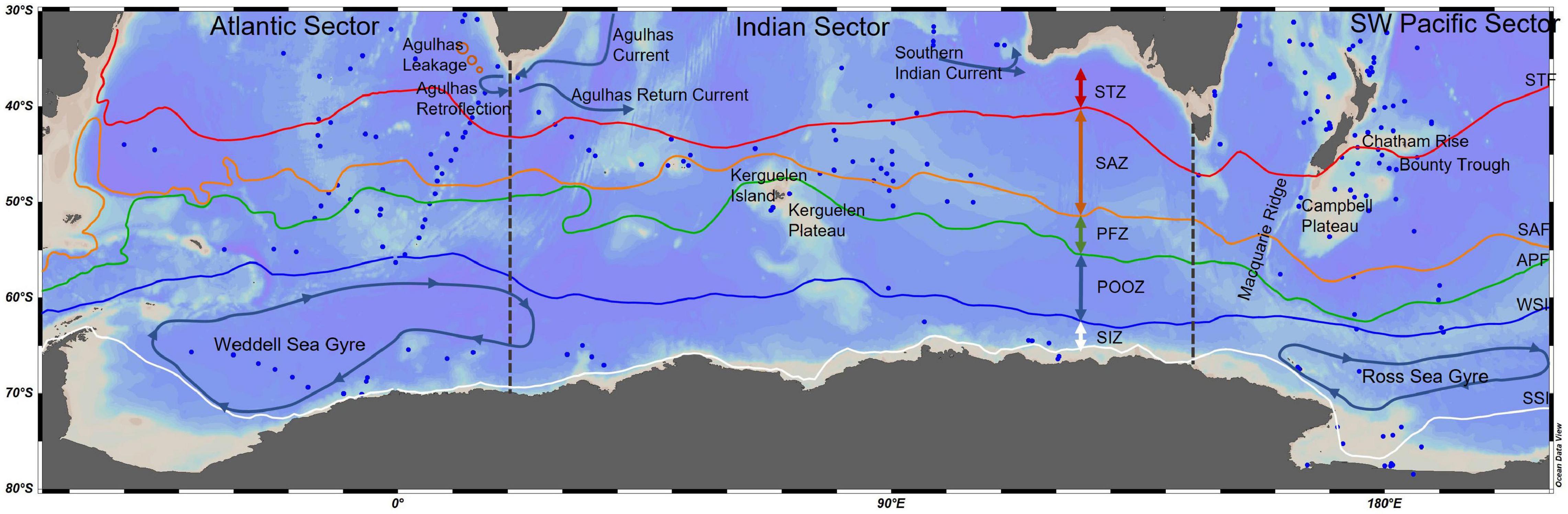
Figure 1. Southern Ocean map showing the location of surface sediment sites of the SO-RAD database (Lawler et al., 2021) south of 30°S within each sector of the Southern Ocean. Major topographical and hydrological features discussed in this paper and the division between three Sectors – Atlantic, Indian and Southwest Pacific. Hydrological fronts [STF (red), Subtropical Front; SAF (orange), Subantarctic Front; APF (green), Antarctic Polar Front; Orsi et al., 1995] and zones (STZ, Subtropical Zone; SAZ Subantarctic Zone; PFZ, Polar Frontal Zone; POOZ, Permanently Open Ocean Zone; SIZ, Seasonal Sea-Ice Zone), summer and winter sea-ice margins [WSI (blue), Winter Sea-Ice Margin; SSI (white), Summer Sea-Ice Margin], major Eastern Boundary Currents and the two major gyres – Weddell Sea and Ross Sea Gyres. Blue arrows depict regional currents and gyres, and direction of flow.

Our main aim is to examine the extent of radiolarian assemblage heterogeneity throughout the SO and how it might be linked to oceanographic and biogeochemical variability. Understanding the heterogeneity and relationship between specific oceanographic regions and the radiolarian assemblages that inhabit those regions is critical for understanding radiolarian ecology and environmental preferences to aid the interpretation of paleo-environmental changes from preserved radiolarian assemblages in sediment cores from the SO.

Materials and Methods

Background

Radiolarians

Since their first description by Ehrenberg (1844), between 400 and 800 living species of radiolarians have been identified (Boltovskoy and Correa, 2016; Boltovskoy, 2017). With a high level of species diversity and robust skeletons that are generally well preserved in the sedimentary record, radiolarians are valuable tools for paleo-studies (e.g., Cortese et al., 2007; Aitchison et al., 2017).

Radiolarian species distribution is influenced by properties of water masses and related frontal systems (Abelmann and Gowing, 1997). Some species and groups have been associated with specific depths and regions, which suggests they might have water mass preferences (e.g., Abelmann and Gowing, 1997; Cortese and Prebble, 2015; Zoccarato et al., 2016). Assemblage distribution is also known to be strongly related to temperature (Boltovskoy and Correa, 2016). Methods for reconstructing sea surface temperatures (SST) were developed which applied factor analysis and transfer functions for paleotemperature estimates throughout the SO (Imbrie and Kipp, 1971; CLIMAP, 1976, 1981; Cortese et al., 2013; Panitz et al., 2015; Prebble et al., 2017; Civel-Mazens et al., 2021b). Radiolarians have also been used as indicators for upwelling in some tropical regions, where characteristic assemblages have been utilized to understand past upwelling processes. Indices such as the Upwelling Radiolarian Index and the Water Depth Ecology Index rely on either the presence of radiolarian species that are typically only found in regions of upwelling, or higher than normal abundance of species that typically inhabit the water column below the thermocline (Caulet et al., 1992; Nigrini and Caulet, 1992; Lazarus et al., 2006).

Southern Ocean Setting

The SO surrounds Antarctica and is the only circumpolar ocean on the globe. It is dominated by the eastward flowing wind-driven ACC (Rintoul and Naveira Garabato, 2013). The STF marks the northern-most extent of ACC influence, and for the purpose of this paper, we define the STF as the northern boundary of the SO (Talley et al., 2011). The SO is most commonly described in terms of three major latitudinal zones which are bounded by hydrological fronts (Figure 1; Orsi et al., 1995). The SAZ sits between the STF and the Subantarctic Front (SAF). The Polar Frontal Zone (PFZ) lies between the SAF and the Polar Front (PF). South of the PFZ is the Antarctic Zone (AZ) (Sokolov and Rintoul, 2009). Within the AZ, sea ice expands and contracts seasonally within the SIZ. During summer, sea ice contracts to the Summer Sea-Ice Margin. South of the Summer Sea-Ice Margin, sea-ice cover remains relatively permanent, except in some coastal regions where no sea-ice is present during summer (polynyas). Seasonal sea-ice expansion extends to the Winter Sea Ice (WSI) margin, beyond which lies the permanently open ocean zone (POOZ) (Pondaven et al., 2000; Talley et al., 2011).

Regions within the SO are often referenced to in relation to the adjacent basin. There are three major geographical regions, the Atlantic Sector (65°W to 20°E), the Indian Sector (20–145°E) and the Pacific Sector (145°E to 65°W) (Lawler et al., 2021). However, in this study, the Pacific is referred to as the Southwest Pacific (145°E to 170°W) due to the limited coverage of data in the Pacific sector within the SO-RAD (Lawler et al., 2021).

Southern Ocean Radiolarian Dataset

The Southern Ocean Radiolarian Dataset (SO-RAD) is a collection of 228 Holocene surface sediment samples from the Atlantic, Indian and Southwest Pacific Sectors of the SO (Figure 1; Lawler et al., 2021). Site locations range from the STZ to the AZ. The SO-RAD contains a total of 238 taxonomic units. Identification level is predominantly to subspecies/species level, though ranges through to orders Nassellaria and Spumellaria (Lawler et al., 2021). The data was cleaned prior to analyses by removing counts for taxa that were classified to class or order only. Those taxa removed totaled less than 10% relative abundance for 80% of sites, and never more than 30% relative abundance for all other sites. No rare species were removed prior to analyses so that potentially significant rare species could be investigated. When assessing SO heterogeneity only the SAZ, PFZ, and AZ SO-RAD sites were included. Sector-specific analyses included sites south 30°S in the STZ to understand the assemblage variability between SO Sectors (Atlantic, Indian and Southwest Pacific) and their adjacent basins.

Some zones and regions of the SO are underrepresented, or not represented at all, within the SO-RAD database. The most notable of such regions is the Southeast Pacific Sector. The PFZ of the SW Pacific and Indian Sectors, southern Australian region, and western Indian Sector are also underrepresented. The SO-RAD database will continue to be updated as further data become available and the addition of data from these regions will allow us to fill in the geographical gaps that currently exist in our analyses and results. Despite these limitations, this is the first and most complete circumpolar surface sediment radiolarian dataset currently available.

Environmental Data

Environmental data representing the climatological mean between 1955 and 2010, including nutrient and density data, were extracted from World Ocean Atlas 2018 0.25 and 1.0 degree grids for Austral summer months of January to March (Garcia et al., 2019). We used data at intervals between 0 and 500 m for nutrient, temperature and salinity data, and between 0 and 2,000 m for density data, as radiolarians are known to inhabit the water column down to these depths (Boltovskoy, 2017). Mixed Layer Depth (variable density) data (MLD-vd) for Austral summer (JFM) and winter (JAS) were extracted from Global Ocean Mixed Layer Depths (Monterey and Levitus, 1997). All data extraction was performed in Ocean Data View v5.4.0 (Schlitzer, 2020).

Data Analysis

All data analyses were performed using the open source software program R (R Core Team, 2018).

Hellinger dissimilarity distance was calculated for the SO-RAD database abundances (Legendre and De Cáceres, 2013). This method addresses two considerations when analyzing radiolarian datasets. Radiolarians are typically counted to a maximum number of individuals per sample (usually between 400 and 500 individuals), so counts vary considerably but are not equivalent to absolute abundance. The second consideration is the high frequency of zero counts. Many zeros in a dataset can result in the double zero problem: similarity is calculated to be higher between sites that have fewer species present, even if they contain no species in common (Legendre and De Cáceres, 2013).

Non-metric Multidimensional Scaling

Ecoregionalisation is commonly used to understand how community structure changes over a larger region. The first step in this process is to identify ecological patterns in the radiolarian assemblages (Grant et al., 2006). Since radiolarian ecology is relatively unknown, an unconstrained method is used, independent of environmental parameters, allowing us to understand distribution patterns without prior knowledge of any ecological drivers. The nMDS method represents the dissimilarity of objects in a small number of dimensions (usually two or three). The objective is to produce a visual representation of dissimilarity in space, rather than preserving the exact relationships in all dimensions, as with metric scaling. The degree to which the plot represents the dissimilarity in the original matrix is shown by the stress value, between 0 and 1. A lower stress value points to a more representative plot of the dissimilarity matrix (Legendre and Legendre, 2012). The nMDS can be applied to any distance matrix. Here we apply it to the Hellinger distance matrix.

The Hellinger-transformed species data was used to perform 2- and 3-dimensional nMDS using the R Package ‘vegan’ (Oksanen et al., 2019). Two- and three-dimensional ordination plots were produced to visualize the patterns of assemblage dissimilarity with the R packages ‘ggplot2’ (Wickham, 2016) and ‘rgl’ (Adler and Murdoch, 2020).

The resulting nMDS plots display the best representation of dissimilarity between each point, or site, relative to all the others, providing a visualization of the trends in assemblage composition (Figure 2). Clustering of points on nMDS plots indicates relative similarity between them, while greater distance indicates relative dissimilarity. The plots are able to show gradients of change as well as distinct and very dissimilar groups. To understand where the delineation is between groups, cluster analysis (in this case, Multivariate Regression Tree) allows us to decide where thresholds of compositional change occur. Together, these two methods provide a comprehensive tool for examining the structure of an ecological community.

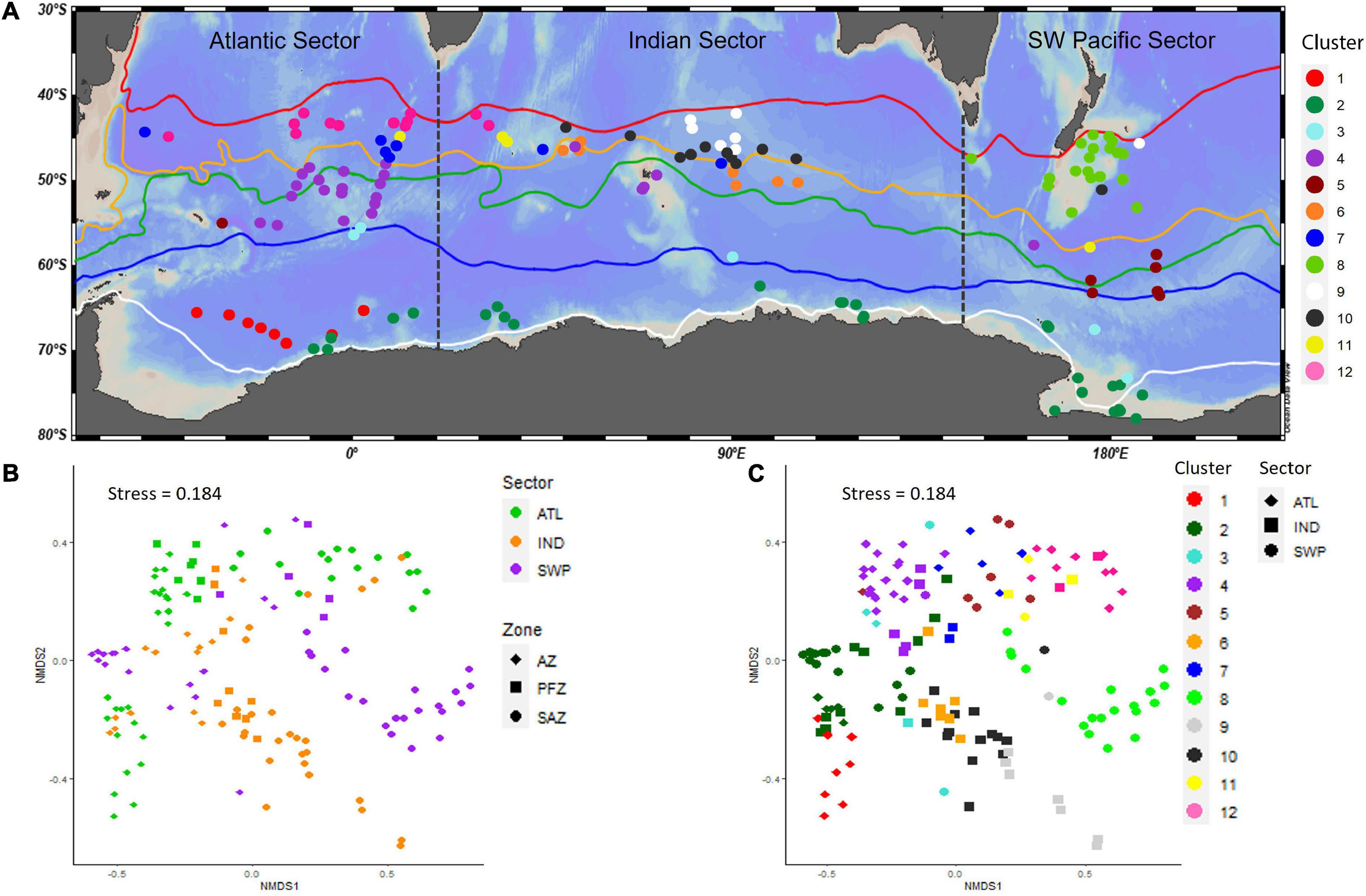
Figure 2. Sites of the SO-RAD with the Southern Ocean from the Subtropical Front to the Antarctic Zone. (A) Map of distribution of clusters determined by MRT analysis of sites within the Southern Ocean; STF, Subtropical Front; SAF, Subantarctic Front; APF, Antarctic Polar Front (Orsi et al., 1995); STZ, Subtropical Zone; SAZ, Subantarctic Zone; PFZ, Polar Frontal Zone; POOZ, Permanently Open Ocean Zone; SIZ, Seasonal Sea-Ice Zone; WSI, Winter Sea-Ice Margin; SSI, Summer Sea-Ice Margin. (B) nMDS of Hellinger transformed relative abundance of Southern Ocean sites. Shape depicts the zone: Antarctic Zone (AZ), Polar Frontal Zone (PFZ), and Subantarctic Zone (SAZ). Color depicts sector: ATL, Atlantic Sector; IND, Indian Sector; SWP, Southwest Pacific. (C) nMDS as per (B), color depicting MRT clusters and shape depicting Sector. Please see Supplementary Figure 1 for a color blind alternative.

Multivariate Regression Tree Analysis

We followed the procedure of De’Ath (2002) to undertake an MRT analysis, a method of partitioning a response variable (in this case, species abundance) based on a set of explanatory variables. This method partitions the response data into two groups that each contain sites with the lowest possible dissimilarity. Partitioning is then repeated for the two subgroups. The analysis output provides the optimal number of clusters for the study based on minimized relative error, and the cross validated relative error. Multiple iterations of the process are performed, indicating the number of times different numbers of clusters are determined to be optimal, and that best case number of clusters can then be preselected for the final analysis. The result is a tree where splits, or nodes, represent environmental thresholds and the end members represent the clusters (De’Ath, 2002; Borcard et al., 2018). Clustering using MRT has the advantage of being a robust method capable of determining clusters where there is a high level of interaction between the explanatory variables (as is usually the case in an oceanic setting), even where there are missing values (Borcard et al., 2018).

The Hellinger transformed species and environmental data were used to perform MRT analysis using the R package ‘mvpart’ (Therneau et al., 2013). Results of the MRT analysis were extracted using the R package ‘MVPARTwrap’ (Ouellette and Legendre, 2014). The R code was adapted from Borcard et al. (2018). The MRT procedure was performed on each subset as outlined in Section “Spatial Variability in SO-RAD Assemblages.” Once clusters were determined using the MRT procedure, these were plotted on maps of the SO to visualize patterns of radiolarian assemblage distribution.

In contrast to nMDS plots that display unconstrained view (i.e., variability seen in the species abundance data alone) of dissimilarity in species data, MRT provides a constrained view (i.e., the assemblage variability that can be explained by the environmental variables) of the dissimilarity. In this paper’s context, MRT clusters confirm site similarity seen in nMDS plots and allow us to determine connectivity and ecoregion boundaries based on how the environmental variables affect the dissimilarity observed in the species data alone. These two methods have been used individually or together in many marine ecosystem studies including microplankton (e.g., Rogers and De Deckker, 2007; Kortsch et al., 2012; Armbrecht et al., 2014; Armynot du Châtelet et al., 2018). The MRT analysis results were compared to those of hierarchical clustering for validation of the MRT clusters.

Redundancy Analysis

While the MRT uses response variables to determine clusters of sites with similar assemblage composition, the RDA seeks to determine how much influence the combinations of explanatory, or environmental variables have on the assemblage. The method attempts to find a series of linear combinations of explanatory variables through multivariate regression and computes these as canonical axes. The order of the RDA axes relates to the amount of constrained or explained variability in the response data, with the first having the highest canonical eigenvalue and explanatory power, while all unconstrained variability is expressed as residual eigenvalues (Borcard et al., 2018). The proportion of variance explained by each RDA axis is equivalent to the coefficient of determination (R²). This is a biased figure, and so an adjusted R² should be calculated (Peres-Neto et al., 2006). There are a number of assumptions about the data used for RDA, for example, the normal distribution of response variables (Borcard et al., 2018). Ecological data such as community composition rarely meet these criteria, so a permutation test is needed to check the overall significance of the RDA results (Borcard et al., 2018). Here we tested all environmental variables in a single RDA to assess how the species abundance data can be explained by all the environmental variables, and if a single or small group of variables showed strong explanatory value. We then tested each variable individually to assess how much influence each variable has on the species abundance data. The RDA was performed on the Hellinger-transformed species data using the R package ‘vegan’ function rda(), and the adjusted R² was calculated using the function RsquareAdj() (Oksanen et al., 2019). A global permutation test of the full RDA results, and a permutation test of the canonical axes were performed, both with 999 permutations, using function anova(). The first constrained (RDA1) and unconstrained (PC1) eigenvalues were used to calculate the lambda ratio (λ₁/λ₂). This ratio assists in determining which environmental parameters show important gradients, a value higher than 1, meaning the first constrained axis (RDA1) explains more variance than the first unconstrained axis (PC1; Juggins, 2013). Those explanatory variables with a lambda ratio greater than 1 (λ₁/λ₂ > 1) were selected for a partial RDA and subjected to permutation tests for global and axis significance.

Results

Spatial Variability in SO-RAD Assemblages

Southern Ocean

Two- and three-dimensional (2D and 3D) nMDS plots of radiolarian assemblages of the SO (SAZ to AZ) showed that different basins (e.g., the South Atlantic, Indian and SW Pacific Sectors) were generally identifiable (Figures 2, 3). When all sites were visualized together, the variability of sites from north to south within each Sector plotted along a different plane. This was particularly evident in the 3D nMDS (stress = 0.093), indicating assemblages in each Sector do not vary in the same fashion and are likely responding to different drivers. Each Sector was then subsplit into oceanographic zones (Figure 2). A general north-south trend was apparent in the 2D nMDS (stress = 0.184), with SAZ sites furthest from AZ sites for all sectors, indicating greatest dissimilarity.

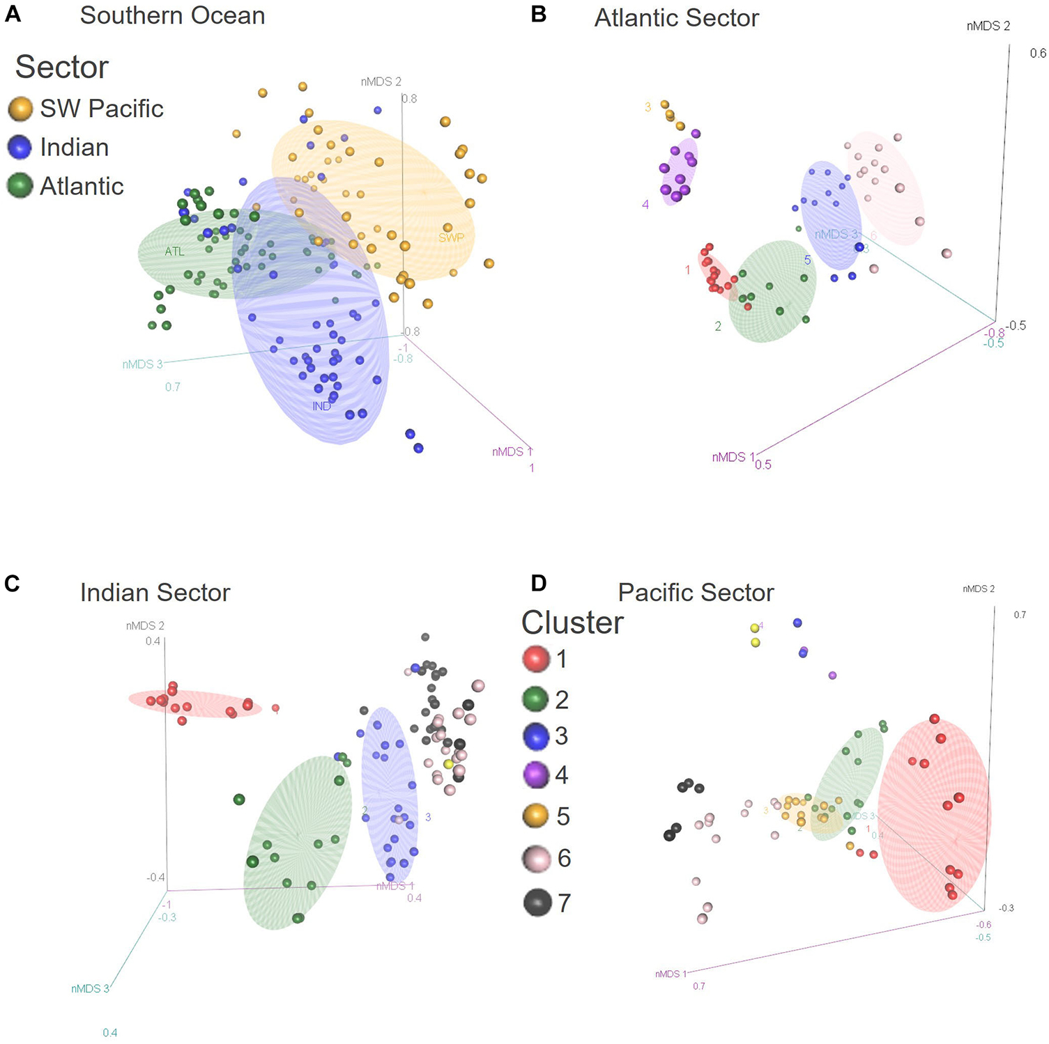
Figure 3. Three dimensional NMDS plots for Hellinger transformed radiolarian assemblage data at sites of the SO-RAD database south of 30°S for the (A) Southern Ocean, (B) Atlantic, (C) Indian, and (D) Pacific Sectors. Colors represent (A) sectors and (B–D) the ecoregions identified by MRT analysis.

The nMDS plots (Figure 2) showed a transition in site assemblage composition from the Atlantic to Indian SAZ. As expected, due to their contiguity, sites located furthest to the west in the Indian Sector plotted close to Atlantic Sector SAZ sites, indicating that these sites host similar assemblages. The dissimilarity between Indian and Atlantic sites increased for each site moving further east into the Indian Sector, indicating a transition in assemblage composition from the Atlantic to Indian Sector.

The MRT analysis confirmed the heterogeneity of radiolarian assemblages identified by the nMDS plot (Figure 2) and provided 12 clusters with unique radiolarian assemblages (Table 1). Each Sector contained a unique combination of clusters, with only 4 of the 12 occurring in all three Sectors (clusters 2, 3, 4, and 11). Three clusters (1, 6, and 8) occurred only once, in the Weddell Sea (cluster 1), the Indian PFZ (cluster 6) and the Campbell Plateau (cluster 8). Clusters 11 and 12 overlapped the Atlantic-Indian Sector boundary and confirmed that there is a transition and connectivity of assemblages from the Atlantic to Indian Sectors (Figure 2). The sites in the SIZ formed two distinct clusters – one in the Weddell Sea Gyre, and one along the Antarctic Coast and Shelf (ACS). Some overlap of these two clusters occurred on the eastern boundary of the Weddell Sea.

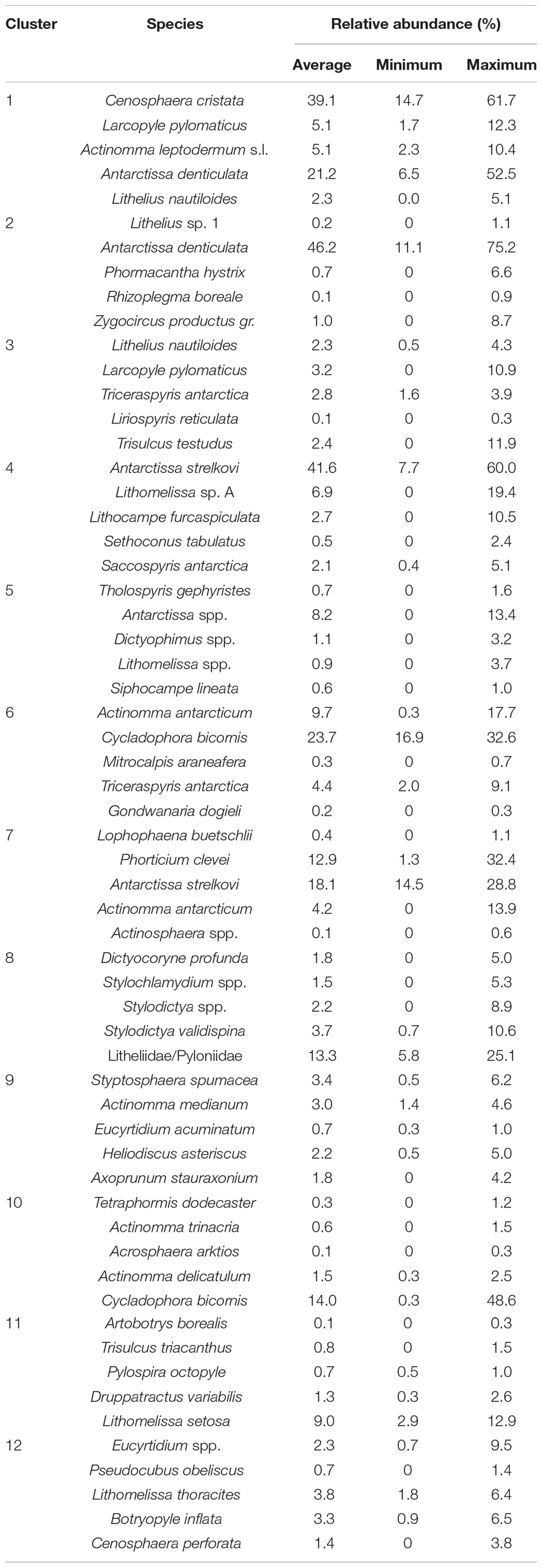
Table 1. The top five species that contribute each cluster of the Southern Ocean Multivariate Regression Tress analysis, and their average, maximum, and minimum relative abundance across all sites that occur in the cluster.

Each Sector had more than one cluster of sites within the AZ. Sites on the western boundary of the Indian Sector clustered with Atlantic Sector AZ sites, and sites on the eastern boundary of the Indian Sector clustered with SW Pacific sites located at the WSI margin. Atlantic AZ sites clustered in two groups – one associated with the SIZ, the other group contained sites located in the POOZ. Within the Pacific Sector, two groups of sites clustered together – sites in the POOZ, and sites in the SIZ. While sites in the SIZ plot with an east-west trending transition on the nMDS, the MRT analysis shows that they should be grouped as a single ecoregion. While each Sector contained more than one cluster within the SIZ, the ACS was common to all sectors.

The SO analyses identified strong primary partitioning at the Sector level, and so it is appropriate to consider each Sector separately for mesoscale ecoregionalisation. In the following sections, we present the results of the analyses of each Sector individually. Here, the clusters are shown as ecoregions, and we use colloquial names for them, describing their relationship to geographical features, for ease of reading the text (these are annotated on Figure 4). The association of the ecoregion with the geographical feature does not denote any environmental connection. The Antarctic Coast and Shelf sites are considered a single ecoregion, and are discussed in each Sector as the Antarctic Coastal and Shelf (ACS) Ecoregion.

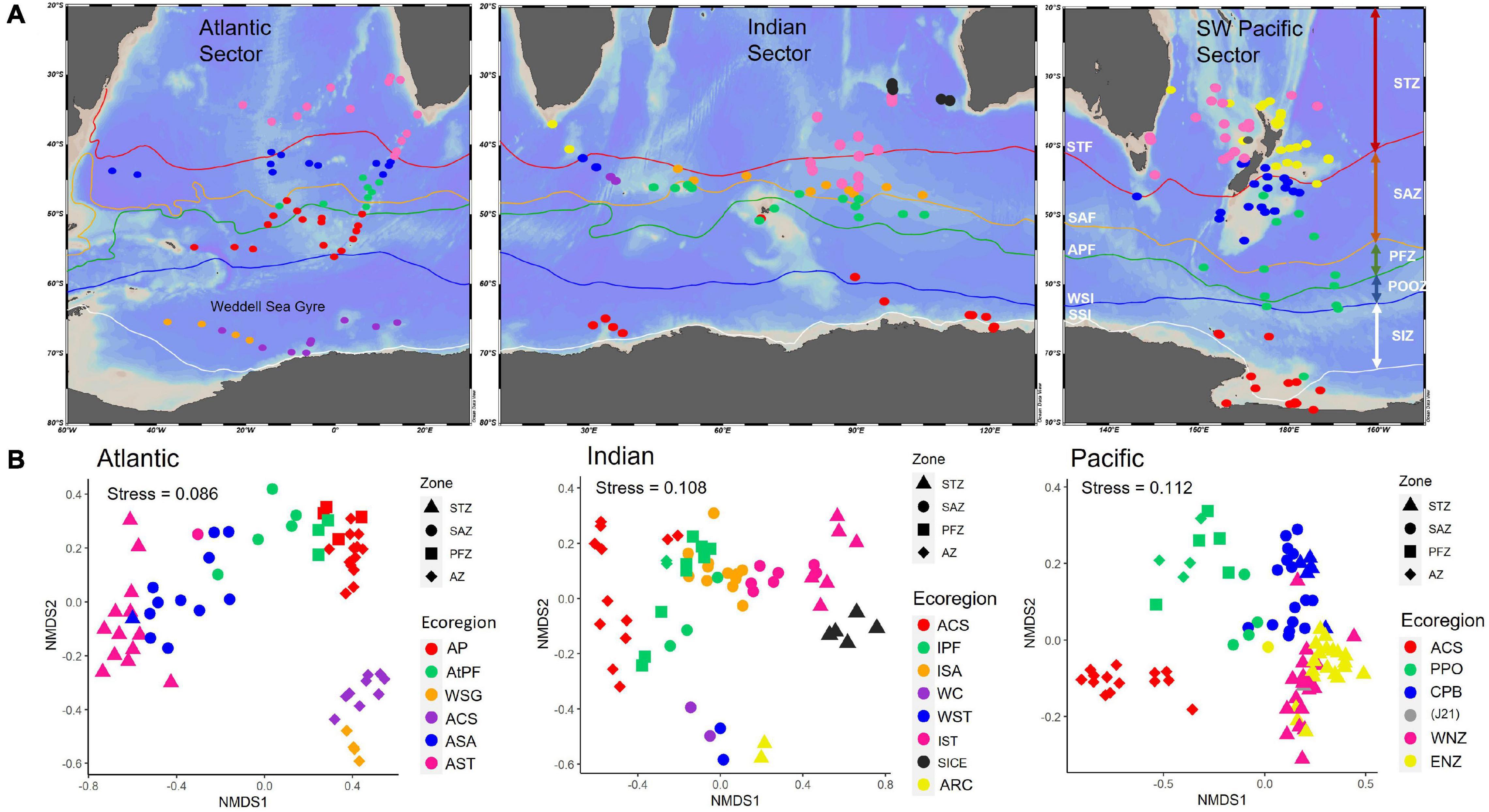
Figure 4. (A) Maps show the distribution of sites within ecoregions identified by the MRT analysis for each Sector. STF, Subtropical Front; SAF, Subantarctic Front; APF, Antarctic Polar Front (Orsi et al., 1995); STZ, Subtropical Zone; SAZ, Subantarctic Zone; PFZ, Polar Frontal Zone; POOZ, Permanently Open Ocean Zone; SIZ, Seasonal Sea-Ice Zone; WSI, Winter Sea-Ice Margin; SSI, Summer Sea-Ice Margin. (B) 2-dimensional NMDS plots for Hellinger transformed radiolarian assemblage data at sites of the SO-RAD dataset south of 30°S for the Atlantic, Indian and Pacific Sectors. Color represents the ecoregions identified by MRT analysis; shapes represent the zone: STZ, Subtropical Zone; SAZ, Subantarctic Zone; PFZ, Polar Frontal Zone; AZ, Antarctic Zone. Pease see Supplementary Figure 2 for a color blind alternative.

Atlantic Sector

Sites within the Atlantic Sector SO-RAD subset showed a distinct north-south trend in assemblage composition in the 2D (stress = 0.086) and 3D (stress = 0.048) nMDS plots (Figures 3, 4). Assemblages at sites in the SIZ were most distinct from all other sites, their dissimilarity apparent by their relative distance from other sites on both plots (Figures 3, 4).

The MRT analysis provided boundaries to the north-south transition of assemblages visible on the Atlantic Sector nMDS (Figure 4; Atlantic Sector map symbol color in brackets). Some sites that are located near frontal boundaries were clustered by MRT analysis with the adjacent zone, rather than its allocated zone according to the Orsi fronts (Figure 4; Orsi et al., 1995). This could be related to the dynamic nature of hydrological fronts. The single mean position of the fronts does not display the extent of frontal shifts, and is therefore considered a guide only for oceanographic boundaries.

North of the STF, the Atlantic Subtropical Ecoregion (pink) encompassed all STZ sites. South of the STF, the clear north-south trend roughly corresponded to the frontal zones: with the Atlantic Subantarctic Ecoregion (blue) between the SAF and PF, the Atlantic Polar Frontal Ecoregion (green) south of the Antarctic Polar Front, and the Atlantic POOZ Ecoregion (red) north of the WSI. South of the WSI margin, two ecoregions were associated with the Weddell Sea Gyre (orange) and the ACS (purple) ecoregions. A single site that was classified within the ACS occurred within the Weddell Sea Gyre. However, this site was grouped with the Weddell Sea Gyre in the SO MRT analysis (Figure 2), reflecting that the assemblage is a transition between these two.

Indian Sector

Indian Sector assemblages vary according to a north-south trend in both the 2D (stress = 0.108) and 3D (stress = 0.062) nMDS plots (Figures 3, 4). There is a group of six sites located in the western Indian Sector that are dissimilar to other sites within the STZ and SAZ. The four sites within the SAZ were found to cluster in SO MRT analysis with sites immediately to the west within the Atlantic Sector. Their positions on the 2D and 3D nMDS plots show that their similarity to assemblages in the Indian Sector increases to the east (Figures 3, 4). MRT analysis confirms that they are distinct from the rest of the Indian Sector assemblages. These formed three ecoregions (Figure 4, Indian Sector map symbol color in brackets) – The Agulhas and Return Current (yellow), the Indian Western STF (blue), and the Western Crozet (purple) Ecoregions.

In the eastern Indian Sector, a group of sites from the South Indian Current area forms an ecoregion (gray). A cluster extending from the STZ to SAZ is the Indian STZ Ecoregion (pink). Within the PFZ and SAZ, two groups extend from west to east, with a narrow latitudinal extent and are roughly divided by the SAF – the Indian PFZ Ecoregion (green) and the Indian SAZ Ecoregion (orange). The clusters within this STZ to the PFZ area east of the Kerguelen Plateau are similar to those found by Rogers and De Deckker (2007), who also used MRT to perform cluster analysis in the same region.

Sites within the SIZ plot with an east-west trending transition. However, MRT analysis shows that they should be grouped as a single ecoregion, the ACS (red).

SW Pacific Sector

The 2D (stress = 0.112) nMDS showed a general north-south trend for sites north of the WSI margin. North of the STF, the 2D and 3D (stress = 0.0725) nMDS plots indicated that assemblages transition toward the SAZ. The MRT analysis showed that these sites can be roughly partitioned according to their location east or west of the North Island of New Zealand – the East and West New Zealand Ecoregions. Sites located on the Campbell Plateau and in the Bounty Trough grouped together, and the MRT analysis confirmed that these sites form the Campbell Plateau Ecoregion. Assemblages appeared on the nMDS to transition from the West New Zealand Ecoregion (pink) to the East New Zealand Ecoregion (yellow) and then to the Campbell Plateau Ecoregion (blue). A single site, Station Site J21 (gray), was identified by MRT analysis, but was indistinct on the nMDS.

Within the POOZ, from the WSI margin to the flanks of the Campbell Plateau, there was a gradient in assemblage composition from south to north on the nMDS, but not enough to provide a partitioning by the MRT analysis. This group was classified as the Pacific POOZ Ecoregion (green). South of the WSI margin, a distinct cluster of sites within the AZ was found on the nMDS. These sites are located within the ACS (red).

Environmental Drivers

The first two constrained eigenvalues of the RDA using the SO subset with all environmental variables accounted for 45% of the total constrained variance [Eigenvalue (proportion explained), RDA 1 = 0.1219 (0.2459), RDA 2 = 0.1001 (0.2018); adjusted R² = 0.60; anova (global), F = 3.1582, P = 0.001]. No single or small group of explanatory variables were clear controls on the data. When analyzing each individual variable with RDA, 17 variables were eliminated based on low explanatory power (λ₁/λ₂ < 1; Table 2). The adjusted R² values for the remaining variables (λ₁/λ₂ > 1) ranged from 0.16 to 0.19. These variables were included in a partial RDA. The first two constrained eigenvalues of the partial RDA accounted for 33.5% of the total constrained variance [Table 3; Eigenvalue (proportion explained), RDA 1 = 0.1108 (0.2055), RDA 2 = 0.0697 (0.1292); adjusted R² = 0.54; anova (global), F = 5.8673, P = 0.001]. The partial RDA revealed that a complex combination of abiotic variables drives radiolarian assemblage data, and no single variable could be identified alone as a clear control.

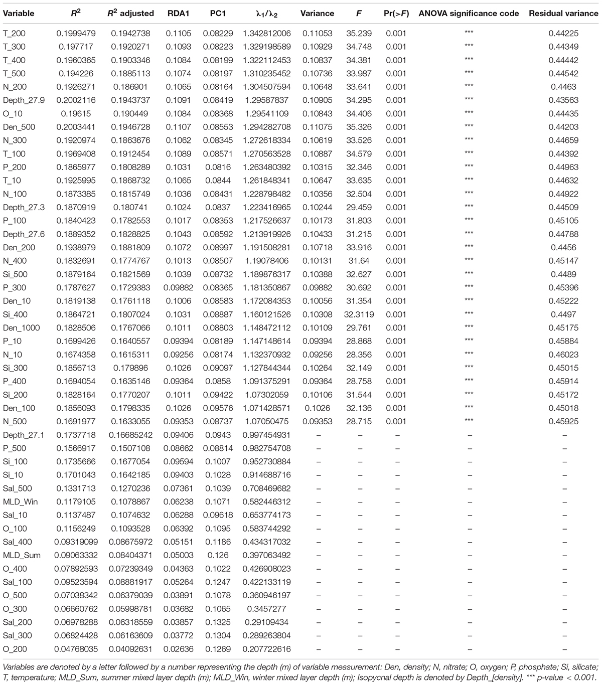
Table 2. List of environmental variables used for individual redundancy analysis and Lambda (λ₁/λ₂) selection for partial redundancy analysis.

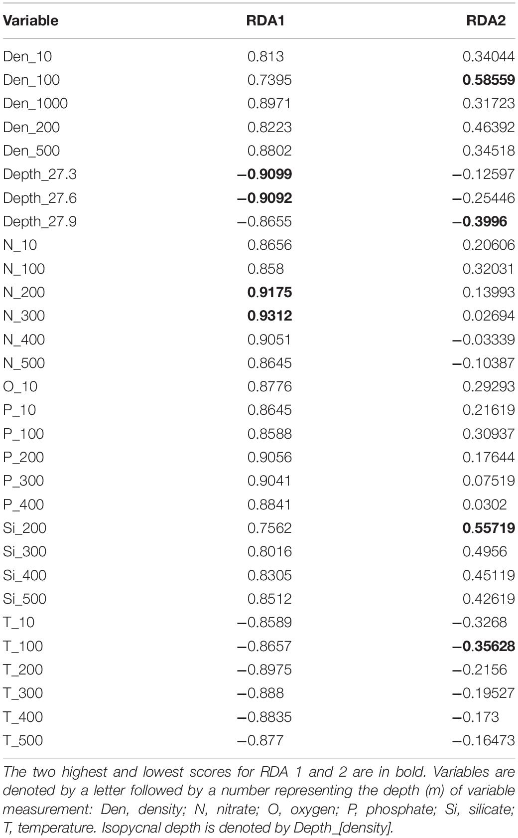
Table 3. Environmental variable RDA scores for Lambda (λ₁/λ₂) selected variables used in a partial redundancy analysis.

Discussion

Heterogeneity of the Southern Ocean

Radiolarian assemblages of the SO-RAD surface sediment census dataset (Lawler et al., 2021) were found to be heterogeneous both latitudinally and longitudinally. We expected the assemblages to vary latitudinally due to strong associations between radiolarian assemblages and sea surface and sub-surface temperature, one of the main reasons why radiolarians have typically been used as temperature proxies (Abelmann et al., 1999; Cortese and Abelmann, 2002; Panitz et al., 2015; Civel-Mazens et al., 2021b). However, if temperature were the only driver of radiolarian distribution, we would expect to see homogeneity of assemblage composition along isotherms, which are characteristically longitudinal throughout the SO. Previous radiolarian work has tended to focus on a single region or Sector at a time. Here, for the first time, we have been able to show the longitudinal and Sector variations using the SO-RAD database (Lawler et al., 2021) and highlight that each Sector of the SO hosts unique radiolarian communities.

Our results show that radiolarian distribution can be divided according to Sector, each containing a distinct assemblage and unique pattern of north-south trending variability. The exception to this Sector variation is in the SO-RAD assemblages found south of the WSI margin in the AZ. Here, the assemblages show greater similarity than those north of the WSI margin, apart from sites within the Weddell Sea Gyre. Nishimura and Nakaseko (2011) also reported a typical Antarctic pelagic radiolarian assemblage throughout the SO south of 60°S within the SIZ.

This longitudinal heterogeneity of the radiolarian assemblages is somewhat unexpected, as previous work on SO species including fish and echinoids, showed a very different pattern of species distribution (Koubbi et al., 2010; Fabri-Ruiz et al., 2020), with an increase of homogeneity moving away from the shelf region to the open ocean. The increase in habitat complexity and diversity in the benthic realm approaching the Antarctic shelf and coastal regions may contribute to the increased diversity in the benthos in those regions. González-Wevar et al. (2018) noted that even species with very low dispersal potential are found to have a remarkably homogeneous distribution throughout the SAZ. The authors remark that the flow of the ACC may have resulted in lower assemblage heterogeneity north of the PF compared to the AZ by providing a mechanism for dispersal and high levels of circumpolar connectivity, even for species with low dispersal potential. Radiolarians are purely planktonic organisms and appear to have the opposite relationship between communities north and south of the WSI margin. The extremes of environmental conditions south of the WSI margin at the highest SO latitudes may provide environmental pressures that reduce species diversity, leading to less variability in assemblages. Along the coastal and shelf regions, the water mass conditions are comparatively more stable throughout the year than north of the WSI margin. This is likely the result of changes in the properties of water within the ACC on its circumpolar path due to the entrainment and upwelling of various other water masses (western boundary currents, North Atlantic Deep Water, Indian Deep Water, Pacific Deep Water, Upper Circumpolar Deep Water, etc.). The surface waters are also influenced by topographical influences on frontal system locations and interactions (e.g., cross frontal eddies, frontal merging and splitting of the main ACC jets, i.e., front has multiple jets N-SAF, S-SAF, N-PF, and S-PF; Lumpkin and Speer, 2007).

Attempts to determine which environmental variables drive the distribution of SO radiolarians using the RDA suggests that no single or small group of variables are the main drivers of the patterns observed in this study. This is likely due to the collinearity of many variables in the SO. Therefore, radiolarians do not appear to respond to a single variable, but rather a combination. Previous work using radiolarians as a proxy for temperature appear robust (Cortese et al., 2013; Panitz et al., 2015; Prebble et al., 2017; Civel-Mazens et al., 2021b) suggesting that temperature has a strong influence on the distribution of radiolarians (Boltovskoy and Correa, 2016; Hernández-Almeida et al., 2017). Furthermore, the use of radiolarian indices for oceanographic features such as upwelling and water masses have also shown potential, for example the Upwelling Radiolarian Index and Water Depth Ecology index (Lazarus et al., 2006; Nigrini and Caulet, 1992). Exploring the relationship between radiolarians and other environmental parameters could allow for the development of other proxies or indices useful for understanding species/assemblage ecology and paleoceanography of the SO.

Heterogeneity Within Each Sector

Since each Sector hosts a unique distribution of radiolarian assemblages, it is important to examine each one separately. Here we will discuss the features that appear to be associated with the distribution of radiolarians, and potential drivers of the patterns we observed in each Sector.

Atlantic Sector

The Atlantic Sector provides no significant topographical obstacle to the flow of the ACC east of the Drake Passage and the East Scotia Ridge. The clear north-south trend of radiolarian distribution reflects this relative simplicity. The assemblages from the SIZ are quite distinct from those in the POOZ, indicating that sea ice processes are a potential driver of radiolarian distribution. Within the SIZ, there are two variations of radiolarian composition: one includes sites within the Weddell Gyre; the other is associated with Antarctic shelf areas.

The Weddell Gyre has several processes that could account for the unique assemblage that occurs in the SIZ, which are different from those affecting the assemblages found associated with the open Antarctic Coast and Shelf regions. The cyclonic Weddell Gyre results in strong upwelling of nutrient-rich deep water. The gyre is also influenced by ice sheet meltwater and calved icebergs from the Filchner–Ronne Ice Shelf flow into the Weddell Sea from shelf streams. The resuspension of shelf sediments and the melting of icebergs are all thought to bring significant quantities of the limiting micronutrient iron (Fe) to the Weddell Gyre (Graham et al., 2015). The interactions of these unique features result in high primary productivity, and may contribute to the unique radiolarian assemblages that occur here (Vernet et al., 2019). Boltovskoy and Alder (1992) noted that radiolarian assemblages in the Weddell Gyre occurred at greater depths (peak at 240 m), where Warm Deep Water lies, than in other AZ regions. They also noted that the assemblages in the Weddell Gyre contained subtropical radiolarian species that likely traced the path of the Warm Deep Water from lower latitudes, all of which could explain the unique assemblage of the Weddell Gyre.

Indian Sector

The main feature highlighted by the Indian Sector nMDS plot was a distinct group of radiolarian assemblages at sites where the Agulhas and Agulhas Return Currents flow around the southern tip of the African continent. These two currents form the strongest, most variable western boundary system across the world’s oceans (Thompson, 2012; Zhu et al., 2018). The Agulhas Current is a Western Boundary Current in the upper 800 m of the water column that brings warm Indian Ocean water poleward along the east coast of the African continent (Lutjeharms, 2006). After reaching the southern tip of Africa, the current turns at the Agulhas Retroflection, where it begins shedding mesoscale eddies (Lutjeharms and Ansorge, 2001). Westward traveling eddies result in some leakage of Western Boundary Current water into the South Atlantic Ocean (Lutjeharms, 2006; Graham and De Boer, 2013). However, most of the flow turns eastward, forming the Agulhas Return Current, which reaches down to around 3,000 m depth, crossing the Agulhas and Mozambique Plateaux (Lutjeharms, 2006). There is strong decadal to millennial modulation of variability in the intensity of this system, and so is likely important for driving variability in radiolarian assemblages across glacial cycles (Timmermann, 2003). The eddies formed by the Agulhas Return Current play a role in transporting heat from the warm Agulhas Retroflection and Agulhas Return Current to the relatively cooler surrounding waters. The radiolarian assemblages located here were distinct from the other Indian Sector assemblages, indicating that these currents are potential drivers of the Indian Sector’s west-east heterogeneity.

Assemblages downstream of the Crozet and Kerguelen Islands in the PFZ and SAZ are distinct from other regions. The presence of eddy fields, the proximity of frontal systems to each other and shallow topography may contribute to this distinction. Eddy pumping in this region entrains deep nutrient-rich water and brings it to the surface resulting in high primary productivity (Dawson et al., 2018). The limiting micro-nutrient Fe is released during the resuspension of shelf sediments via the shelf pump and transported eastward by the ACC frontal jets, and southward via cross-frontal eddy transport (Blain et al., 2008; Graham et al., 2015; Resplandy et al., 2019; Uchida et al., 2020). Civel-Mazens et al. (2021a,b) suggested that changes in eddy kinetic energy and Fe concentrations in this region east of the Kerguelen Plateau can be seen in the downcore radiolarian assemblages over glacial cycles. During the Holocene and interglacials, it was proposed that the ACC and frontal jets interacted more with the Kerguelen Plateau, increasing mixing, nutrient supply and primary productivity. Higher eddy kinetic energy during the current interglacial may account for the Indian PFZ Ecoregion seen downstream of the Crozet and Kerguelen Islands. There is a distinct Ecoregion shift from upstream to downstream of Crozet Island (map colors: purple upstream to green downstream). However, there is a lack of data upstream of Kerguelen Island for an assessment of this hypothesis.

SW Pacific Sector

The nMDS plot for the SW Pacific Sector reveals that assemblage composition varies in relation to topographical features, which strongly control the position and flow of the region’s frontal systems and currents. North of the STF in the low nutrient, warm subtropical waters, the assemblages appear relatively similar, but there are distinct assemblages east and west of the North Island of New Zealand. A potential candidate for the differentiation between assemblages in the STZ is the East Australian Current, which leaves the Australian coast and flows east across the Tasman Sea in the Tasman Front via a series of stationary eddies then around the top of the North Island of New Zealand (Stanton et al., 1997; Hill et al., 2011).

The Chatham Rise, which locks the position of the STF to its southern flank (Chiswell et al., 2015), acts as a divide between the NE subtropical and the Campbell Plateau Ecoregion. A distinct ecoregion was associated with the Campbell Plateau, SW of New Zealand, a large, relatively shallow plateau less than 1,000 m deep (Figure 1). The depth of the Campbell Plateau may exclude the typical deep-living radiolarians, and the Campbell Plateau Ecoregion would therefore stand out from the nearby assemblages in regions of much deeper bathymetry, such as the POOZ ecoregion. More recent work on SO hydrographic fronts (e.g., Sokolov and Rintoul, 2009; Park et al., 2019) show that the Campbell Plateau steers the SAF around it’s flank compared to the proposed SAF position of Orsi et al. (1995). When considering the more recently proposed positions of the SAF, the Campbell Plateau Ecoregion forms a coherent SAZ assemblage (Figure 4, blue cluster). Subantarctic Mode Water and Antarctic Intermediate Water are present over the Campbell Plateau and Bounty Trough, respectively (Forcén-Vázquez et al., 2021). The steep slope of the Campbell Plateau directs the flow of the full depth SAF around its south-eastern flank (Chiswell et al., 2015; Forcén-Vázquez et al., 2021). Previous work also found a similar pattern of radiolarian distribution in the Southwest Pacific region using factor analysis to show links to water mass associations in this region (Cortese and Prebble, 2015). The boundaries of partitioning from factor analysis were very similar to those found using MRT clustering in this study, further supporting these ecoregions.

A distinct assemblage was found to extend from the south-eastern boundary of the Campbell Plateau to the WSI margin. This represents a region of ice-free ocean that has relatively deep and flat topography (abyssal plains), dominated by the strong flowing ACC. The potential influence of the Macquarie Ridge, which focuses the flow of the ACC through narrow gaps and generates significant downstream eddy activity, was not clear in this study, as the SO-RAD does not currently include sites immediately west of the ridge.

A distinct assemblage within the SIZ in the Southwest Pacific Sector was easily identified on the nMDS plot. Most of these sites are within the Ross Sea. Seasonal sea-ice formation and melt within the Ross Sea result in large fluctuations in the abiotic properties of the water column, including nutrient concentrations, irradiance, temperature and salinity (Smith and Comiso, 2008; Smith et al., 2012). The dynamics associated with sea ice processes are known to impact diatom assemblages, resulting in high productivity during spring and into summer (Ferry et al., 2015; Rajanahally et al., 2015). High primary productivity is further promoted by polynya activity (Pinkerton et al., 2020). The same environmental controls that influence diatom and other phytoplankton assemblages may also play a role in affecting the species composition of radiolarian assemblages. Furthermore, the high availability of food resources due to the large diatom blooms on the Ross Sea Shelf may additionally affect radiolarian assemblage composition and abundance. Zoccarato et al. (2016) also found that the mixing and transformation of water masses in this region that lead to the formation of the very dense shelf water of the Ross Sea, influenced the composition and abundance of the Ross Sea protist community (including radiolarians).

Other Drivers of Heterogeneity

The alteration of water properties due to the upwelling and mixing of different water masses, along with the local influences of increased bioavailable Fe concentrations, which likely influence the phytoplankton communities which radiolarians consume, may influence the association between radiolarian assemblages and the characteristic oceanographic features of the Sectors. Each Sector receives water from the adjacent ocean basins, which carries with it a unique suite of properties (Lumpkin and Speer, 2007). The mixing of these different water properties may produce enough variability between Sectors to result in Sector-specific radiolarian assemblage distribution. Despite the uninterrupted eastward flowing ACC, the localized water property alterations may explain why that connectivity does not translate into a continuous longitudinal zone of homogeneous radiolarian assemblage composition. This alteration to assemblages resulting from altered water mass properties was previously observed by Zoccarato et al. (2016). The study found that eukaryotic communities, including radiolarians, in Antarctic Bottom Water at the Ross Sea shelf break, had the assemblage signature of its parent water masses, entrained Circumpolar Deep Water and shelf water.

Two Indian Sector clusters, the Indian PFZ and Indian SAZ, may be related to different levels of Fe availability. Natural Fe fertilization results in high primary productivity, as it is a limiting micronutrient in the High Nutrient-Low Chlorophyll SO (Uchida et al., 2020). Fe fertilization occurs in regions where mesoscale eddy activity transports Fe to surface waters from the deep, particularly downstream of islands and shallow topography, or where ice-melt and runoff introduce Fe to the water column in coastal regions (Graham et al., 2015; Ellwood et al., 2020; Uchida et al., 2020). While a direct association between radiolarians and Fe has not yet been found, the resulting increase in primary productivity may increase food resources and impact radiolarian assemblage composition, distribution, and abundance.

Ecological interactions, such as competition and predator-prey interactions, have significant impacts on community structure. Other zooplankton such as copepods and ostracods are known to occupy similar space in the water column as radiolarians, specifically at the base of the mixed layer, where a deep chlorophyll maximum can occur, along with the accumulation of detritus from surface waters (Lima-Mendez et al., 2015). Thus, an additional factor affecting the radiolarian assemblage distribution could be the absence or presence of other zooplankton species. Some radiolarians are colonial and have symbiotic relationships with algae and dinoflagellates, creating a complex intra- and interspecific inter-dependence that may influence assemblage composition (Suzuki and Not, 2015). The ecological interactions and tolerances of their symbionts can also influence the distribution of radiolarians.

Here we do not suggest causation of radiolarian distribution in the SO, but rather discuss the features that coincide with the observed patterns of SO-RAD radiolarian distribution. Future work should explore environmental and ecological factors that may drive the heterogeneity found in this study, as well as the ecological impact of radiolarian assemblage variation on the larger ecosystem.

Comparison to Bioregionalisation of the Southern Ocean

The results of this study did not contradict the latitudinal zones that were previously proposed for SO bioregions. However, our results indicated that the SO can be divided by Sectors and further subdivided by the latitudinal zones (Figures 3, 4). Testa et al. (2021) presented physical and biogeochemical regionalization models, the former resulting in homogeneous latitudinal bands, while the latter presented a complex pattern of regions that varied significantly between Sectors. The results of this study support the complexity presented by the latter. However, radiolarian distribution appears less complex than the patterns observed by Testa et al. (2021) suggesting that radiolarians are not as sensitive to the fine-scale variability used to define the biogeochemical regions.

Application of SO-RAD Ecoregions

A goal of eco- and bioregionalisation is to determine environmental drivers of assemblage groups for defining different ecologically distinct regions, which may be important for the proposal of Marine Protected Areas and protecting biodiversity. Additionally, they can be used to reconstruct past conditions – paleoceanography. This ecoregionalisation study shows that radiolarian assemblages differ between SO Sectors based on the SO-RAD database. The heterogeneity between SO Sectors and the lack of close connection evident in the nMDS and the MRT indicate that each Sector has a unique radiolarian assemblage likely as a response to a unique and complex combination of environmental drivers. Therefore, only census data from the relevant Sector should be used as a modern analog in paleo-environmental studies from that Sector.

Conclusion

The SO-RAD database allows a first assessment of radiolarian assemblages across three Sectors of the Southern Ocean. The use of nMDS combined with MRT cluster analysis to identify dissimilarity across the SO has shown both latitudinal and longitudinal variation in radiolarian assemblages. The longitudinal heterogeneity, especially within the ACC, where homogeneity would have been expected due to connectivity of flow and similar SST conditions, is surprising. Each Sector is host to a unique composition of radiolarian assemblages, transitioning from one Sector to another and forming a distinct pattern of ecoregions. These differences are likely driven by variability in the oceanographic characteristics of each Sector, and this variation must be considered when studying radiolarian ecology or using them for paleo-reconstructions in the SO.

Data Availability Statement

Publicly available datasets were analyzed in this study. This data can be found here: https://github.com/vloweSO/SO-Radiolarian-Ecoregionalisation.

Author Contributions

VL performed the analyses and wrote the initial version of the manuscript. GC and HB reviewed and provided support for analyses, interpretations, and revision of the initial manuscript. All authors contributed to the results, interpretations, and successive versions of the manuscript.

Funding

VL and K-AL are each supported by an Australian Research Training Program (RTP) scholarship. GC contribution was supported by the New Zealand Ministry of Business, Innovation and Employment through the Antarctic Science Platform (ANTA1801) and the Global Change through Time Programme (GCT SSIF, contract C05X1702).

Conflict of Interest

The authors declare that the research was conducted in the absence of any commercial or financial relationships that could be construed as a potential conflict of interest.

Publisher’s Note

All claims expressed in this article are solely those of the authors and do not necessarily represent those of their affiliated organizations, or those of the publisher, the editors and the reviewers. Any product that may be evaluated in this article, or claim that may be made by its manufacturer, is not guaranteed or endorsed by the publisher.

Acknowledgments

We wish to thank the reviewers for their valuable comments that allowed us to enhance the manuscript.

Supplementary Material

The Supplementary Material for this article can be found online at: https://www.frontiersin.org/articles/10.3389/fmars.2022.829676/full#supplementary-material

Supplementary Figure 1 | Sites of the SO-RAD with the Southern Ocean from the Subtropical Front to the Antarctic Zone. (A) Map of distribution of clusters (1–12) determined by MRT analysis of sites within the Southern Ocean; STF, Subtropical Front; SAF, Subantarctic Front; APF, Antarctic Polar Front (Orsi et al., 1995); STZ, Subtropical Zone; SAZ, Subantarctic Zone; PFZ, Polar Frontal Zone; POOZ, Permanently Open Ocean Zone; SIZ, Seasonal Sea-Ice Zone; WSI, Winter Sea-Ice Margin; SSI, Summer Sea-Ice Margin. (B) nMDS of Hellinger transformed relative abundance of Southern Ocean sites. Shape depicts the zone: Antarctic Zone (AZ), Polar Frontal Zone (PFZ), and Subantarctic Zone (SAZ). Shade depicts sector: ATL, Atlantic Sector; IND, Indian Sector; SWP, Southwest Pacific. (C) nMDS as per (B), shade depicting sector clusters and numbers (1–12) depicting MRT cluster.

Supplementary Figure 2 | (A) Maps show the distribution of sites within ecoregions identified by the MRT analysis for each Sector. STF, Subtropical Front; SAF, Subantarctic Front; APF, Antarctic Polar Front (Orsi et al., 1995); STZ, Subtropical Zone; SAZ, Subantarctic Zone; PFZ, Polar Frontal Zone; POOZ, Permanently Open Ocean Zone; SIZ, Seasonal Sea-Ice Zone; WSI, Winter Sea-Ice Margin; SSI, Summer Sea-Ice Margin. (B) 2-dimensional NMDS plots for Hellinger transformed radiolarian assemblage data at sites of the SO-RAD dataset south of 30°S for the Atlantic, Indian and Pacific Sectors. Color represents the ecoregions identified by MRT analysis; shapes represent the zone: STZ, Subtropical Zone; SAZ, Subantarctic Zone; PFZ, Polar Frontal Zone; AZ, Antarctic Zone. Key associated with each Sectors’ nMDS also refers to the associated map above.

References

Abelmann, A., Brathauer, U., Gersonde, R., Sieger, R., and Zielinski, U. (1999). Radiolarian-based transfer function for the estimation of sea surface temperatures in the Southern Ocean (Atlantic Sector). Paleoceanography 14, 410–421.
Abelmann, A., and Gowing, M. M. (1997). Spatial distribution pattern of living polycystine radiolarian taxa - baseline study for paleoenvironmental reconstructions in the Southern Ocean (Atlantic sector). Mar. Micropaleontol. 30, 3–28.
Adler, D., and Murdoch, D. (2020). Package ‘rgl.’ Available online at: https://CRAN.R-project.org/package=rgl (accessed April 14, 2020).
Aitchison, J. C., Suzuki, N., Caridroit, M., Danelian, T., and Noble, P. (2017). Paleozoic radiolarian biostratigraphy. Geodiversitas 39, 503–531. doi: 10.5252/g2017n3a5
Ardyna, M., Claustre, H., Sallée, J. B., D’Ovidio, F., Gentili, B., van Dijken, G., et al. (2017). Delineating environmental control of phytoplankton biomass and phenology in the Southern Ocean. Geophys. Res. Lett. 44, 5016–5024. doi: 10.1002/2016GL072428
Armbrecht, L. H., Roughan, M., Rossi, V., Schaeffer, A., Davies, P. L., Waite, A. M., et al. (2014). Phytoplankton composition under contrasting oceanographic conditions: upwelling and downwelling (Eastern Australia). Cont. Shelf Res. 75, 54–67. doi: 10.1016/j.csr.2013.11.024
Armynot du Châtelet, E., Francescangeli, F., Bouchet, V. M. P., and Frontalini, F. (2018). Benthic foraminifera in transitional environments in the English Channel and the southern North Sea: a proxy for regional-scale environmental and paleo-environmental characterisations. Mar. Environ. Res. 137, 37–48. doi: 10.1016/j.marenvres.2018.02.021
Be, A. W. H., and Tolderlund, D. S. (1971). “Distribution and ecology of living plankton Foraminifera in surface waters of the Atlantic and Indian Oceans,” in The Micropaleontology of Oceans, eds B. M. Funnel and W. R. Riedel (Cambridge: Cambridge University Press), 105–159.
Blain, S., Sarthou, G., and Laan, P. (2008). Distribution of dissolved iron during the natural iron-fertilization experiment KEOPS (Kerguelen Plateau. Deep Sea Res. II Top. Stud. Oceanogr. 55, 594–605. doi: 10.1016/j.dsr2.2007.12.028
Boltovskoy, D. (2017). Vertical distribution patterns of Radiolaria Polycystina (Protista) in the World Ocean: living ranges, isothermal submersion and settling shells. J. Plankton Res. 39, 330–349. doi: 10.1093/plankt/fbx003
Boltovskoy, D., and Alder, V. A. (1992). Paleoecological implications of radiolarian distribution and standing stocks versus accumulation rates in the Weddell Sea. Antarct. Res. Ser. 56, 377–384. doi: 10.1029/ar056p0377
Boltovskoy, D., and Correa, N. (2016). Biogeography of Radiolaria Polycystina (Protista) in the World Ocean. Prog. Oceanogr. 149, 82–105. doi: 10.1016/j.pocean.2016.09.006
Borcard, D., Gillet, F., and Legendre, P. (2018). Numerical Ecology with R, 2nd Edn. Cham: Springer.
Caulet, J. P., Vénec-Peyré, M. T., Vergnaud-Grazzini, C., and Nigrini, C. (1992). “Variation of South Somalian upwelling during the last 160 ka: radiolarian and foraminifera records in core MD 85674,” in Upwelling Systems: Evolution since the Early Miocene, eds C. P. Summerhayes et al. (London: Special Publications), 379–389. doi: 10.1144/GSL.SP.1992.064.01.25
Chiswell, S. M., Bostock, H. C., Sutton, P. J. H., and Williams, M. J. (2015). Physical oceanography of the deep seas around New Zealand: a review. N. Z. J. Mar. Freshw. Res. 49, 286–317. doi: 10.1080/00288330.2014.992918
Civel-Mazens, M., Crosta, X., Cortese, G., Michel, E., Mazaud, A., Ther, O., et al. (2021b). Impact of the Agulhas Return Current on the oceanography of the Kerguelen Plateau region. Quat. Sci. Rev. 251:106711. doi: 10.1016/j.quascirev.2020.106711
Civel-Mazens, M., Crosta, X., Cortese, G., Michel, E., Mazaud, A., Ther, O., et al. (2021a). Antarctic Polar Front migrations in the Kerguelen Plateau region, Southern Ocean, over the past 360 kyrs. Glob. Planet. Change 202:103526. doi: 10.1016/j.gloplacha.2021.103526
CLIMAP (1976). The surface of the ice-age Earth. Science 191, 1131–1137. doi: 10.1126/science.191.4232.1131
CLIMAP (1981). Seasonal Reconstruction of the Earth’s Surface at the Last Glacial Maximum. Boulder, CO: Geological Society of America.
Cortese, G., and Abelmann, A. (2002). Radiolarian-based paleotemperatures during the last 160 kyr at ODP Site 1089 (Southern Ocean. Palaeogeogr. Palaeoclimatol. Palaeoecol. 182, 259–286. doi: 10.1016/S0031-0182(01)00499-0
Cortese, G., Abelmann, A., and Gersonde, R. (2007). The last five glacial-interglacial transitions: a high-resolution 450,000-year record from the subantarctic Atlantic. Paleoceanography 22, 1–14. doi: 10.1029/2007PA001457
Cortese, G., Dunbar, G. B., Carter, L., Scott, G., Bostock, H., Bowen, M., et al. (2013). Southwest Pacific Ocean response to a warmer world: Insights from marine isotope stage 5e. Paleoceanography 28, 585–598. doi: 10.1002/palo.20052
Cortese, G., and Prebble, J. (2015). A radiolarian-based modern analogue dataset for palaeoenvironmental reconstructions in the southwest Pacific. Mar. Micropaleontol. 118, 34–49. doi: 10.1016/j.marmicro.2015.05.002
Dawson, H. R. S., Strutton, P. G., and Gaube, P. (2018). The unusual surface chlorophyll signatures of southern ocean eddies. J. Geophys. Res. Oceans 123, 6053–6069. doi: 10.1029/2017JC013628
De’Ath, G. (2002). Multivariate regression trees: a new technique for modeling species-environment relationships. Ecology 83, 1105–1117.
Ehrenberg, C. G (1844). On microscopic life in the ocean at the South Pole, and at considerable depth. Ann. Mag. Nat. Hist. 14, 169–181. doi: 10.1080/037454809496376
Ellwood, M. J., Strzepek, R. F., Strutton, P. G., Trull, T. W., Fourquez, M., and Boyd, P. W. (2020). Distinct iron cycling in a Southern Ocean eddy. Nat. Commun. 11:825. doi: 10.1038/s41467-020-14464-0
Fabri-Ruiz, S., Danis, B., Navarro, N., Koubbi, P., Laffont, R., and Saucède, T. (2020). Benthic ecoregionalization based on echinoid fauna of the Southern Ocean supports current proposals of Antarctic Marine Protected Areas under IPCC scenarios of climate change. Glob. Change Biol. 26, 2161–2180. doi: 10.1111/gcb.14988
Ferry, A. J., Crosta, X., Quilty, P., Fink, D., Howard, W. I., and Armand, L. K. (2015). First records of winter sea ice concentration in the southwest Pacific sector of the Southern Ocean. Paleoceanography 23, 1525–1539. doi: 10.1002/2014PA002764
Forcén-Vázquez, A., Williams, M. J. M., Bowen, M., Carter, L., and Bostock, H. (2021). Frontal dynamics and water mass variability on the Campbell Plateau. N. Z. J. Mar. Freshw. Res. 55, 199–222. doi: 10.1080/00288330.2021.1875490
Garcia, H. E., Boyer, T. P., Baranoba, R. A., Locarnini, A. V., Mishonov, A., Grodsky, A., et al. (2019). World Ocean Atlas 2018. NOAA National Centers for Environmental Infomation. Available online at: https://accession.nodc.noaa.gov/NCEI-WOA18 (accessed 24, 2021).
González-Wevar, C. A., Segovia, N. I., Rosenfeld, S., Ojeda, J., Hüne, M., Naretto, J., et al. (2018). Unexpected absence of island endemics: long-distance dispersal in higher latitude sub-Antarctic Siphonaria (Gastropoda: Euthyneura) species. J. Biogeogr. 45, 874–884. doi: 10.1111/jbi.13174
Graham, R. M., and De Boer, A. M. (2013). The dynamical subtropical front. J. Geophys. Res. Oceans 118, 5676–5685. doi: 10.1002/jgrc.20408
Graham, R. M., De Boer, A. M., van Sebille, E., Kohfeld, K. E., and Schlosser, C. (2015). Inferring source regions and supply mechanisms of iron in the Southern Ocean from satellite chlorophyll data. Deep Sea Res. I Oceanogr. Res. Pap. 104, 9–25. doi: 10.1016/j.dsr.2015.05.007
Grant, S., Constable, A., Raymond, B., and Doust, S. (2006). Bioregionalisation of the Southern Ocean: Report of Experts Workshop. Hobart: WWF-Australia and ACE CRC.
Hernandez-Almeida, I., Boltovskoy, D., Kruglikova, S. B., and Cortese, G. (2020). A new radiolarian transfer function for the pacific ocean and application to fossil records: assessing potential and limitations for the last glacial-interglacial cycle. Glob. Planet. Change 190:103186. doi: 10.1016/j.gloplacha.2020.103186
Hernández-Almeida, I., Cortese, G., Yu, P. S., Chen, M. T., and Kucera, M. (2017). Environmental determinants of radiolarian assemblages in the western Pacific since the last deglaciation. Paleoceanography 32, 830–847. doi: 10.1002/2017PA003159
Hill, K. L., Rintoul, S. R., Ridgway, K. R., and Oke, P. R. (2011). Decadal changes in the South Pacific western boundary current system revealed in observations and ocean state estimates. J. Geophys. Res. Oceans 116:C01009. doi: 10.1029/2009JC005926
Grant, S. M., Hill, S. L., and Fretwell, P. T. (2013). Spatial distribution of management measures, antarctic krill catch and southern ocean bioregions: implications for conservation planning. CCAMLR Sci. 20, 1–19.
Imbrie, J., and Kipp, N. G. (1971). “A new micropaleontological method for quantitative paleoclimatology: application to a late Pleistocene Carribean core,” in Late Cenozoic Glacial Ages, ed. K. K. Turekian (New Haven, CT: Yale University Press), 71–181.
Juggins, S. (2013). Quantitative reconstructions in palaeolimnology: New paradigm or sick science? Quat. Sci. Rev. 64, 20–32. doi: 10.1016/j.quascirev.2012.12.014
Kortsch, S., Primicerio, R., Beuchel, F., Renaud, P. E., Rodrigues, J., Lønne, O. J., et al. (2012). Climate-driven regime shifts in Arctic marine benthos. Proc. Natl. Acad. Sci. U.S.A. 109, 14052–14057. doi: 10.1073/pnas.1207509109
Koubbi, P., Ozouf-Costaz, C., Goarant, A., Moteki, M., Hulley, P. A., Causse, R., et al. (2010). Estimating the biodiversity of the East Antarctic shelf and oceanic zone for ecoregionalisation: example of the ichthyofauna of the CEAMARC (Collaborative East Antarctic Marine Census) CAML surveys. Polar Sci. 4, 115–133. doi: 10.1016/j.polar.2010.04.012
Lawler, K., Cortese, G., Civel-mazens, M., Bostock, H., Crosta, X., Leventer, A., et al. (2021). The Southern Ocean RADiolarian (SO-RAD) dataset: a new compilation of modern radiolarian census data. Earth Syst. Sci. Data 13, 5441–5453. doi: 10.5194/essd-13-5441-2021
Lazarus, D., Bittniok, B., Diester-Haass, L., Meyers, P., and Billups, K. (2006). Comparison of radiolarian and sedimentologic paleoproductivity proxies in the latest Miocene-Recent Benguela Upwelling System. Mar. Micropaleontol. 60, 269–294. doi: 10.1016/j.marmicro.2006.06.003
Legendre, P., and De Cáceres, M. (2013). Beta diversity as the variance of community data: dissimilarity coefficients and partitioning. Ecol. Lett. 16, 951–963. doi: 10.1111/ele.12141
Legendre, P., and Legendre, L. (2012). “Ordination in reduced space,” in Numerical Ecology eds P. Legendre and L. Legendre (Oxford: Elsevier), 425–520. doi: 10.1016/b978-0-444-53868-0.50009-5
Lima-Mendez, A. G., Faust, K., Henry, N., Colin, S., Carcillo, F., Chaffron, S., et al. (2015). Determinants of community structure in the global plankton interactome. Science 348:1262073. doi: 10.1126/science.1262073
Linse, K., Griffiths, H. J., Barnes, D. K. A., and Clarke, A. (2006). Biodiversity and biogeography of Antarctic and sub-Antarctic mollusca. Deep Sea Res. II Top. Stud. Oceanogr. 53, 985–1008. doi: 10.1016/j.dsr2.2006.05.003
Longhurst, A. R. (2007). Ecological Geography of the Sea, 2nd Edn. London: Academic Press. doi: 10.1016/B978-0-12-455521-1.X5000-1
Lumpkin, R., and Speer, K. (2007). Global ocean meridional overturning. J. Phys. Oceanogr. 37, 2550–2562. doi: 10.1175/JPO3130.1
Lutjeharms, J. R. E., and Ansorge, I. J. (2001). The agulhas return current. J. Mar. Syst. 30, 115–138. doi: 10.1016/s0924-7963(01)00041-0
Monterey, G., and Levitus, S. (1997). Climatological Cycle of Mixed Layer Depth in the World Ocean. NOAA Atlas NESDIS 14. Washington DC: U.S. Department of Commerce.
Moore, T. C., Hutson, W. H., Kipp, N., Hays, J. D., Prell, W., Thompson, P., et al. (1981). The biological record of the ice-age ocean. Palaeogeogr. Palaeoclimatol. Palaeoecol. 35, 357–370. doi: 10.1016/0031-0182(81)90102-4
Nigrini, C., and Caulet, J. P. (1992). Late Neogene radiolarian assemblages characteristic of Indo-Pacific areas of upwelling. Micropaleontology 38, 139–164. doi: 10.2307/1485992
Nishimura, A., and Nakaseko, K. (2011). Characterization of radiolarian assemblages in the surface sediments of the Antarctic Ocean. Palaeoworld 20, 232–251. doi: 10.1016/j.palwor.2011.05.002
Oksanen, J., Blanchet, F. G., Friendly, M., Kindt, R., Legendre, P., Mcglinn, D., et al. (2019). vegan: Community Ecology Package. R package version 2.4-2. Available Online at: https://cran.r-project.org/web/packages/vegan/vegan.pdf (accessed April 14, 2020).
Orsi, A. H., Whitworth, T., and Nowlin, W. D. (1995). On the meridional extent and fronts of the Antarctic Circumpolar Current. Deep Sea Res. I Oceanogr. Res. Pap. 42, 641–673. doi: 10.1016/0967-0637(95)00021-W
Ouellette, M.-H., and Legendre, P. (2014). Package ‘MVPARTwrap.’ Available Online at: http://www.r-project.org (accessed April 14, 2020).
Panitz, S., Cortese, G., Neil, H. L., and Diekmann, B. (2015). A radiolarian-based palaeoclimate history of Core Y9 (Northeast of Campbell Plateau, New Zealand) for the last 160 kyr. Mar. Micropaleontol. 116, 1–14. doi: 10.1016/j.marmicro.2014.12.003
Park, Y. H., Park, T., Kim, T. W., Lee, S. H., Hong, C. S., Lee, J. H., et al. (2019). Observations of the Antarctic Circumpolar Current Over the Udintsev Fracture Zone, the Narrowest Choke Point in the Southern Ocean. J. Geophys. Res. Oceans 124, 4511–4528. doi: 10.1029/2019JC015024
Peres-Neto, P. R., Legendre, P., Dray, S., and Borcard, D. (2006). Variation Partitioning of Species Data Matrices: estimation and comparison of fractions. Ecology 87, 2614–2625. doi: 10.1890/0012-9658(2006)87[2614:vposdm]2.0.co;2
Pinkerton, M. H., Décima, M., Kitchener, J. A., Takahashi, K. T., Robinson, K. V., Stewart, R., et al. (2020). Zooplankton in the Southern Ocean from the continuous plankton recorder: distributions and long-term change. Deep Sea Res. I Oceanogr. Res. Pap. 162:103303. doi: 10.1016/j.dsr.2020.103303
Pondaven, P., Ragueneau, O., Tréguer, P., Hauvespre, A., Dezileau, L., and Reyss, J. L. (2000). Resolving the “opal paradox” in the Southern Ocean. Nature 405, 168–172. doi: 10.1038/35012046
Prebble, J. G., Bostock, H. C., Cortese, G., Lorrey, A. M., Hayward, B. W., Calvo, E., et al. (2017). Evidence for a Holocene Climatic Optimum in the southwest Pacific: a multiproxy study. Paleoceanography 32, 763–779. doi: 10.1002/2016PA003065
R Core Team (2018). R: A Language and Environment for Statistical Computing. Vienna: R Foundation for Statistical Computing.
Rajanahally, M. A., Lester, P. J., and Convey, P. (2015). Aspects of resilience of polar sea ice algae to changes in their environment. Hydrobiologia 761, 261–275. doi: 10.1007/s10750-015-2362-6
Resplandy, L., Lévy, M., and McGillicuddy, D. J. (2019). Effects of eddy-driven subduction on ocean biological carbon pump. Glob. Biogeochem. Cycles 33, 1071–1084. doi: 10.1029/2018GB006125
Rintoul, S. R., and Naveira Garabato, A. C. (2013). Dynamics of the southern ocean circulation. Int. Geophys. 103, 471–492.
Rogers, J., and De Deckker, P. (2007). Radiolaria as a reflection of environmental conditions in the eastern and southern sectors of the Indian Ocean: a new statistical approach. Mar. Micropaleontol. 65, 137–162. doi: 10.1016/j.marmicro.2007.07.001
Schlitzer, R. (2020). Ocean Data View. Available Online at: https://odv.awi.de (accessed April 14, 2020).
Smith, W. O., and Comiso, J. C. (2008). Influence of sea ice on primary production in the Southern Ocean: a satellite perspective. J. Geophys. Res. Oceans 113:C05S93. doi: 10.1029/2007JC004251
Smith, W. O. J., Sedwick, P. N., Arrigo, K. R., Ainley, D. G., and Orsi, A. H. (2012). The Ross Sea in a sea of change. Oceanography 25, 90–103. doi: 10.5670/oceanog.2012.80
Sokolov, S., and Rintoul, S. R. (2009). Circumpolar structure and distribution of the antarctic circumpolar current fronts: 2. Variability and relationship to sea surface height. J. Geophys. Res. Oceans 114:C11019. doi: 10.1029/2008JC005248
Stanton, B. R., Sutton, P. J. H., and Chiswell, S. M. (1997). The East Auckland Current, 1994–95. N. Z. J. Mar. Freshw. Res. 31, 537–549. doi: 10.1080/00288330.1997.9516787
Suzuki, N., and Not, F. (2015). “Marine protists: diversity and dynamics,” in Marine Protists: Diversity and Dynamics, eds S. Ohtsuka, T. Suzaki, T. Horiguchi, N. Suzuki, and F. Not (Tokyo: Springer), 1–637. doi: 10.1007/978-4-431-55130-0
Talley, L. D., Pickard, G. L., Emery, W. J., and Swift, J. H. (2011). Descriptive Physical Oceanography: An Introduction, 6th Edn. Boston, MA: Elsevier.
Testa, G., Piñones, A., and Castro, L. R. (2021). Physical and Biogeochemical Regionalization of the Southern Ocean and the CCAMLR Zone 48.1. Front. Mar. Sci. 8:592378. doi: 10.3389/fmars.2021.592378
Therneau, T. M., Atkinson, B., Ripley, B., Oksanen, J., and De’ath, G. (2013). Mvpart: Multivariate Partitioning. R Packag. version 1.6-1. Available Online at: http://cran.rproject.org/ (accessed April 14, 2020).
Thompson, P. R. (2012). Sea Surface Height: A Versitile Climate Variable for Investigations of Decadal Change. Ph.D. thesis. Tampa, FL: University of South Florida.
Timmermann, A. (2003). Decadal ENSO amplitude modulations: a nonlinear paradigm. Glob. Planet. Change 37, 135–156. doi: 10.1016/S0921-8181(02)00194-7
Uchida, T., Balwada, D., Abernathey, R. P., McKinley, G. A., Smith, S. K., and Lévy, M. (2020). Vertical eddy iron fluxes support primary production in the open Southern Ocean. Nat. Commun. 11:1125. doi: 10.1038/s41467-020-14955-0
van der Spoel, S. (1983). A Comparative Atlas of Zooplankton: Biological Patterns in the Oceans. Berlin: Springer-Verlag.
Vernet, M., Geibert, W., Hoppema, M., Brown, P. J., Haas, C., Hellmer, H. H., et al. (2019). The Weddell Gyre, Southern Ocean: present knowledge and future challenges. Rev. Geophys. 57, 623–708. doi: 10.1029/2018RG000604
Wickham, H. (2016). ggplot2: Elegant Graphics for Data Analysis. New York, NY: Springer-Verlag. Available online at: https://ggplot2.tidyverse.org (accessed April 14, 2020).
Zhu, Y., Qiu, B., Lin, X., and Wang, F. (2018). Interannual Eddy Kinetic energy modulations in the agulhas return current. J. Geophys. Res. Oceans 123, 6449–6462. doi: 10.1029/2018JC014333
Keywords: radiolarians, Southern Ocean (SO), ecoregionalisation, oceanography, ecology
Citation: Lowe V, Cortese G, Lawler K-A, Civel-Mazens M and Bostock HC (2022) Ecoregionalisation of the Southern Ocean Using Radiolarians. Front. Mar. Sci. 9:829676. doi: 10.3389/fmars.2022.829676
Received: 06 December 2021; Accepted: 27 January 2022;
Published: 03 March 2022.
Edited by:
Gustavo Fonseca, Federal University of São Paulo, BrazilReviewed by:
Johan Renaudie, Natural History Museum, Berlin (MfN), GermanyAlexander Matul, P.P. Shirshov Institute of Oceanology, Russian Academy of Sciences (RAS), Russia
Demetrio Boltovskoy, Universidad de Buenos Aires, Argentina
Copyright © 2022 Lowe, Cortese, Lawler, Civel-Mazens and Bostock. This is an open-access article distributed under the terms of the Creative Commons Attribution License (CC BY). The use, distribution or reproduction in other forums is permitted, provided the original author(s) and the copyright owner(s) are credited and that the original publication in this journal is cited, in accordance with accepted academic practice. No use, distribution or reproduction is permitted which does not comply with these terms.
*Correspondence: Vikki Lowe, v.lowe@uq.edu.au