Estimation of Ocean Biogeochemical Parameters in an Earth System Model Using the Dual One Step Ahead Smoother: A Twin Experiment
 Tarkeshwar Singh
 François Counillon
 Jerry Tjiputra
 Yiguo Wang
 Mohamad El Gharamti
- 1Nansen Environmental and Remote Sensing Center and Bjerknes Centre for Climate Research, Bergen, Norway
- 2Geophysical Institute, University of Bergen, Bjerknes Centre for Climate Research, Bergen, Norway
- 3NORCE Norwegian Research Centre, Bjerknes Centre for Climate Research, Bergen, Norway
- 4National Center for Atmospheric Research, Boulder, CO, United States
Ocean biogeochemical (BGC) models utilise a large number of poorly-constrained global parameters to mimic unresolved processes and reproduce the observed complex spatio-temporal patterns. Large model errors stem primarily from inaccuracies in these parameters whose optimal values can vary both in space and time. This study aims to demonstrate the ability of ensemble data assimilation (DA) methods to provide high-quality and improved BGC parameters within an Earth system model in an idealized perfect twin experiment framework. We use the Norwegian Climate Prediction Model (NorCPM), which combines the Norwegian Earth System Model with the Dual-One-Step ahead smoothing-based Ensemble Kalman Filter (DOSA-EnKF). We aim to estimate five spatially varying BGC parameters by assimilating salinity and temperature profiles and surface BGC (Phytoplankton, Nitrate, Phosphate, Silicate, and Oxygen) observations in a strongly coupled DA framework—i.e., jointly updating ocean and BGC state-parameters during the assimilation. We show how BGC observations can effectively constrain error in the ocean physics and vice versa. The method converges quickly (less than a year) and largely reduces the errors in the BGC parameters. Some parameter error remains, but the resulting state variable error using the estimated parameters for a free ensemble run and for a reanalysis performs nearly as well as with true parameter values. Optimal parameter values can also be recovered by assimilating climatological BGC observations or sparse observational networks. The findings of this study demonstrate the applicability of the DA approach for tuning the system in a real framework.
1. Introduction
Ocean biogeochemistry (BGC) is an important component of an Earth system model (ESM) for simulating the anthropogenic carbon sinks across the air-sea interface (e.g., Marotzke et al., 2017; Tjiputra et al., 2020). It also simulates critical biophysical feedbacks to the climate system such as phytoplankton short-wave absorption (Jochum et al., 2010) and the production of radiatively-important marine aerosol precursor (Schwinger et al., 2017). Following the emergence of seasonal-to-decadal prediction which shows that the ocean variability can be predicted by up to 10 years in advance (Smith et al., 2007; Keenlyside et al., 2008), a similar initiative has been attempted for ocean biogeochemistry (Séférian et al., 2014; Payne et al., 2017; Lovenduski et al., 2019; Park et al., 2019; Fransner et al., 2020).
The accuracy of biological and chemical process representations in ESMs is crucial for simulating the BGC state and variability as realistically as possible. In current state-of-the-art ESMs, the inorganic chemistry is governed by well defined chemical and thermodynamic formulations. However, the biological process representations such as primary production are more uncertain, which leads to a large bias and inter-model spread in their projections (Bopp et al., 2013; Kwiatkowski et al., 2020). The uncertainty becomes more evident at regional scales (Vancoppenolle et al., 2013), hindering their application for regional impact studies. These uncertainties are associated with empirical parameterisations of the biogeochemical inter-actions, which are linked to the complexities and imperfect descriptions of the ocean physical environment that drives the biological process, among others. Generally, ocean BGC models utilise numerous poorly constrained, spatially and temporally constant parameters to simplify the marine ecosystem complexity. Consequently, the large error in the projections, primarily linked to these inaccurate parameters, limits the reliability of the ecosystem model (Losa et al., 2004). One of the reasons for inaccuracy in these parameters is their static nature. Many studies have proven that resolving space and/or time varying BGC parameters is more relevant in the context of biogeochemical modeling (e.g., Losa et al., 2003; Tjiputra et al., 2007; Mattern et al., 2012; Roy et al., 2012; Doron et al., 2013).
Ocean BGC parameters are often estimated and calibrated in small-scale laboratory experiments, which do not always reflect the large-scale open ocean conditions. Once implemented in the global model, these parameters are generalized (i.e., assumed uniform across the globe for simplicity), and tuned within observational uncertainty to capture the observed large-scale BGC properties, for instance primary production, vertical nutrient gradient, deoxygenation pattern, etc. However, this parameter tuning process often becomes complicated and inefficient when the number of parameters increases so as to represent the increasing complexity of biogeochemical models. Therefore, BGC simulations are often subject to a high level of parametric uncertainty and require an efficient method for optimal tuning of their parameters, particularly those which the model is most sensitive to.
Data assimilation (DA) schemes provide an objective and efficient methodology for parameter estimation by combining observations with a numerical model simulation (Eknes and Evensen, 2002). Particularly, ensemble based sequential DA schemes like the Ensemble Kalman Filter (EnKF) offer a simple but efficient framework for automatic optimisation of model parameters alongside the state variables by simply augmenting them together using “Joint-EnKF” formulation (Anderson, 2001; Annan et al., 2005; Jazwinski, 2007). The EnKF (Evensen, 2003) is based on a Monte Carlo sampling of the state space thereby avoiding model linearization. It updates the prior statistics (mean and covariance of state variables) by assuming Gaussian distributed variables and errors. It is one of the widely used sequential DA schemes in the field of geosciences (e.g., Houtekamer and Mitchell, 2001; Reichle et al., 2002; Counillon et al., 2014). However, the application of the EnKF for parameter estimation of numerical models like BGC is both theoretically and practically challenging. Difficulties are usually related to high dimensions and non-linearity of the models as well as other physical constraints such as the positiveness of the BGC variables and parameters. To elaborate, in a high dimensional model like ocean BGC, the number of unknown model state variables and parameters are larger than the available observations. In this case, the EnKF attempts to solve an underdetermined inverse problem at each DA cycle, where it utilises a small number of observations to estimate an extremely large set of unknowns. This problem is more pronounced when the available observations are limited to the surface only, which is often the case for satellite ocean color observations. Furthermore, BGC tracers and parameters, such as nutrient concentration and phytoplankton exudation rate, are positive quantities and cannot be negative. As such, the Gaussian assumptions made in the EnKF (Losa et al., 2004) are not satisfied. To mitigate this issue, a variable-transform approach called Gaussian anamorphosis (Bertino et al., 2003), has been successfully tested and applied for such application (e.g., Simon and Bertino, 2009; Gharamti et al., 2017a). Another challenging issue is the strongly non-linear behavior that BGC models experience during the spring bloom. The rapid temporal dynamics may create large discrepancies between the observations and the ensemble estimates. For example, few ensemble members might start producing a bloom earlier than the rest of the members, which may create inaccurate state and parameter cross-correlations with a linear analysis update. Such a situation often yields unrealistic updates of parameters. On top of the aforementioned challenges, sampling errors due to limited ensemble sizes are generally unavoidable (Natvik and Evensen, 2003), and can degrade the accuracy of the state and parameters. In short, the traditional joint-EnKF scheme for parameter estimation may suffer from above mentioned limitations that could degrade the filter performance (e.g., Moradkhani et al., 2005; Chen and Zhang, 2006; Wen and Chen, 2006).
Recently, many different analysis algorithms have been developed to tackle the limitations of the traditional joint-EnKF with the aim to estimate dynamically consistent and more accurate model parameters. Wen and Chen (2006) derived a confirming-step (CS-EnKF) where the updated parameters are used to rerun the model and obtain reliable state estimates. Another classical approach, suggested by Moradkhani et al. (2005), is a dual updating scheme (Dual-EnKF) for the state and the parameters using two parallel and inter-active EnKFs, where one acts on the state and the other on the parameters. Both the CS-EnKF and the Dual-EnKF are heuristic in nature and do not maintain the Bayesian consistency of the joint state and parameters estimation problem. A recent work by Gharamti et al. (2015) proposed a one-step-ahead smoothing ensemble scheme (OSA-EnKF), which provides a robust estimation framework while respecting the Bayesian consistency of the problem. The algorithm shares a lot of similarities with the CS- and Dual-EnKF, and further introduces a smoothing character in which future observations are used to constrain current state variables. Gharamti et al. (2017b) applied all four estimation schemes (Joint-, CS-, Dual-, and OSA-EnKF) for optimising poorly constrained ecosystem parameters using a one-dimensional configuration of the Ocean BGC model. They concluded that OSA-EnKF is accurate and reliable compared to the others schemes and it successfully recovers the observed seasonal variability of the ecosystem dynamics. Ait-El-Fquih et al. (2016) further derived a more generalized variant of the OSA scheme, namely dual one-step-ahead smoothing EnKF (DOSA-EnKF), by using a dual updating feature where the state variables undergo both smoothing and analysis steps. Motivated by the promising results of OSA scheme in optimising ecosystem parameters, we utilise the generalized variant of the scheme, i.e., DOSA-EnKF for this study.
Another key ingredient for success is the choice of variables in the state vector such that the use of available observations is maximized and the dynamical consistency is preserved. In a coupled model, observations are available in different compartments (ocean, atmosphere, sea ice, biogeochemistry). A simple approach referred to as weakly coupled data assimilation (WCDA; Penny and Hamill, 2017), assimilates the data independently in their respective components. The other model components adjust to these individual changes dynamically in between the assimilation cycles. Allowing the assimilation to update across model components is expected to outperform WCDA because it would enhance the dynamical consistency of the initial conditions and expand the influence of the observations across its own component (strongly coupled data assimilation, SCDA; Penny and Hamill, 2017; Penny et al., 2019). However, the update would still rely on a linear analysis update step, which can be problematic as coupled covariances include complex, coupled phenomena that can be strongly non-linear. Iterative methods such as the dual one step ahead smoother, can better control the growth of non-linearities. For ocean and biogeochemistry this approximation is reasonable, and it has been shown that cross compartment update were beneficial (Yu et al., 2018).
The present study explores the efficiency and the feasibility of the DOSA-EnKF scheme to optimise BGC parameters within an Earth system model in an idealized perfect (or identical) twin experiment framework (Halem and Dlouhy, 1984). In a perfect twin experiment (or identical twin Observing System Simulation Experiment), observations are constructed from the same model and in this study, the only non-perfect aspects of the model are the parameters to be estimated. It differs from fraternal twin experiments (e.g., Arnold Jr and Dey, 1986; Masutani et al., 2010; Halliwell Jr et al., 2014) where observations are constructed from a model that differs from the model used in the data assimilation experiment. Here, we use the Norwegian Climate Prediction Model (NorCPM; Counillon et al., 2014), which provides the ensemble assimilation framework for Norwegian Earth System Model (NorESM1). We aim to estimate five spatially varying BGC parameters by assimilating salinity and temperature hydrographic profiles and surface BGC (Phytoplankton, Nitrate, Phosphorous, Silicate, and Oxygen) observations in a strongly coupled DA framework—i.e., jointly updating ocean and BGC state-parameters during the assimilation. The five ecosystem parameters were also chosen because they are essential to constrain the observed annual cycle of surface BGC, which has been identified as one of the primary sources of future projection uncertainties (Kessler and Tjiputra, 2016; Goris et al., 2018).
The rest of this article is organized as follows. Section 2 summarizes details of model, assimilation algorithm, and experimental design. Section 3 present and discuss the assimilation results and assessment of parameters estimates. Summary and conclusion of the work are given in Section 4.
2. The Norwegian Climate Prediction Model and the Experimental Design
NorCPM (Counillon et al., 2014) is a climate prediction system that aims to provide seasonal-to-decadal prediction (Kimmritz et al., 2019; Wang et al., 2019; Bethke et al., 2021) and long term climate reanalysis (Counillon et al., 2016). It combines the Norwegian Earth System Model (e.g., NorESM1; Bentsen et al., 2013) with the Ensemble Kalman Filter (Evensen, 2003).
2.1. The Norwegian Earth System Model
The NorESM1 is a global fully coupled system, which is based on the Community Earth System Model version 1.0.3 (CESM1; Vertenstein et al., 2012). Unlike CESM1, NorESM1 uses the atmospheric component from the modified version of Community Atmosphere Model (CAM4-Oslo; Kirkevåg et al., 2013). The ocean physical component of NorESM1 is based on Miami Isopycnic Coordinate Ocean Model (MICOM; Bleck and Smith, 1990; Bleck et al., 1992) but with modified numerics and physics (Bentsen et al., 2012). The ocean BGC compartment in NorESM1 is the Hamburg Oceanic Carbon Cycle (HAMOCC; Maier-Reimer et al., 2005; Tjiputra et al., 2013), which is embedded with the isopycnic MICOM model (Assmann et al., 2010). The other components in the model are adopted in their original form from CESM1, which are the Community Land Model (CLM4; Oleson et al., 2010; Lawrence et al., 2011), the Los Alamos sea ice model (CICE4; Gent et al., 2011; Holland et al., 2012) and with the version 7 coupler (CPL7; Craig et al., 2012).
This study utilizes the medium-resolution version of NorESM1 (Tjiputra et al., 2013). The atmospheric component CAM4 and Land component CLM4 are configured on a horizontal resolution of 1.9° at latitude and 2.5° at longitude (approximately 2° finite volume grid). In the vertical, CAM4 features 26 hybrid sigma-pressure levels with model top at approximately 3 hPa. The ocean MICOM and sea ice CICE4 models have a common horizontal resolution of approximately 1° × 1° with refined grids near the Equator in meridional direction, and in both zonal and meridional direction at high latitudes. MICOM uses 51 isopycnal layers and 2 additional layers for representing the bulk mixed layer with time-evolving thicknesses and densities. The biogeochemical component HAMOCC utilizes the same spatial and temporal resolution as the ocean model.
HAMOCC includes an NPZD-type ecosystem module which was initially implemented by Six and Maier-Reimer (1996). It includes one generic class of phytoplankton, one generic class of zooplankton, three macronutrients (phosphate, nitrate, and silicate), and one micronutrient (dissolved iron). In addition to the ecosystem module, it also prognostically simulates full inorganic carbon chemistry, which includes dissolved inorganic carbon and alkalinity. Other key state variables include oxygen, dissolved organic carbon, particulate organic and inorganic carbon, and biogenic opal. The phytoplankton growth rate in the model is formulated as a function of temperature and light availability (Smith, 1936). The primary production is represented by a prognostic function of phytoplankton growth rate, which is limited by temperature, incoming shortwave radiation, and availability of nutrients. Further details of the HAMOCC can be sought from Tjiputra et al. (2013).
NorESM1 has been shown to capture the major observed modes of climatic variability (Bentsen et al., 2013). Further, many studies have demonstrated that it simulates well ENSO variability and its teleconnection (e.g., Sperber et al., 2013; Bellenger et al., 2014). In Anav et al. (2013), it was demonstrated that observed tropical inter-annual variability in ocean primary production reproduced by NorESM1 is in the top three among 18 ESM's used in their study. Tjiputra et al. (2013) evaluated the mean state of HAMOCC with NorESM and reported that NorESM satisfactorily reproduces many of the observed large scale ocean biogeochemical features.
2.2. The Dual One Step Ahead Smoother
The dual one step ahead smoother (DOSA, Gharamti et al., 2015) is an iterative smoother scheme based on the Ensemble Kalman Filter. The DOSA scheme respects the Bayesian consistency of the problem, and proceeds as shown in Figure 1. Here, we use the Deterministic EnKF (DEnKF) in DOSA. The DEnKF is a square-root (deterministic) formulation of the EnKF that solves the analysis without the need to perturb the observations. It inflates the errors by construction and is intended to perform well in operational applications (Sakov et al., 2012).
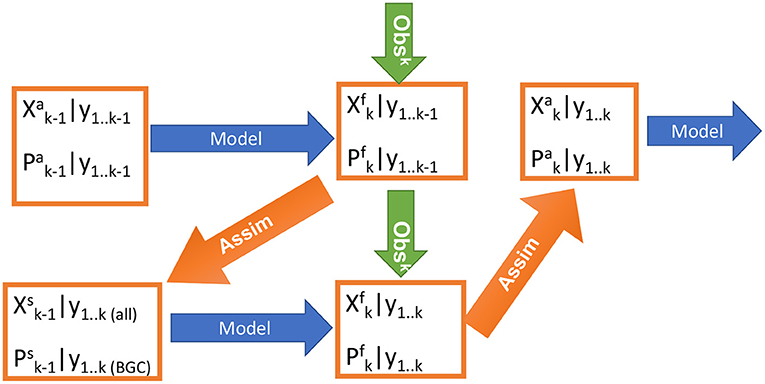
Figure 1. Schematic diagram of the steps of the dual one step ahead (DOSA) scheme.
In the first step, the ensemble of analysed model state and its associated parameters at time k−1, , are integrated forward: =. Note that the parameters are not changed during the model integration (i.e., ).
The observations at time k, yk, are used to produce a smoothed estimate of the state and parameters at the previous analysis step k−1 as follows:
where,
where the superscript T denotes a matrix transpose and A the ensemble anomalies, i.e., , with . In a similar way, the parameter ensemble, , at time k−1 is smoothed using yk.
In the second step, the model is integrated forward to time k again but with smoothed ensemble of state and parameters ; i.e., =.
The observations at time k, yk, are then used again to produce an analysis of
Kk, k is the standard Kalman gain and are the ensemble anomalies constructed from . It should be emphasized that the observations are used twice, but the second time they are used with a model that is using a different set of parameters. As such, model state is updated twice in a assimilation cycle but parameter is updated only at previous time step.
The model state (X) includes several ocean physical and biogeochemical prognostic model variables and they are updated in isopycnal coordinates as in Counillon et al. (2014); Wang et al. (2017). In the physical component, we update the full isopycnal temperature, salinity, layer thickness and velocities (53 isopycnal layers). Similarly, we update the biogeochemical variables at all isopycnal layers which include oxygen, phytoplankton, silicate, nitrate, total dissolved inorganic carbon, total alkalinity, dissolved organic carbon, particulate organic carbon, zooplankton, and biogenic silica. The list of selected BGC parameters for this study is provided in Section 2.3. For the assimilation system, the state vector is composed of the above physical and biogeochemical model variables along with the biogeochemical parameters. When one updates the ocean variable layer thickness, one effectively updates also the mass of the BGC quantities. In Bethke et al. (2021), it was shown that this approach conserves well BGC properties and does not introduce spurious upwelling at the Equator. However, with an EnKF, the linear analysis update returns unphysical values for non-Gaussian distributed variables. Some state variables have a physical constraint and their values should be positive definite such as layer thickness and tracer concentrations. For layer thickness we use the upscaling algorithm (Wang et al., 2016) while for the BGC concentration quantity (i.e., when updating the BGC state) a post-processing step is applied so that negative values are set to zero. We have not noticed degradations caused by the post-processing. We think that it is due to the fact that 1) part of the non-Gaussianity is already handled by the super layer algorithm which updates the layer thickness, and 2) with the smoothing flavor that the DOSA scheme provides, the updated parameters rarely became non-physical (i.e., negative).
Observations are used to update both ocean and BGC components in a strongly coupled framework (Penny and Hamill, 2017). The BGC component does not feedback to the physics in this version of NorESM and thus error in the physical state cannot be caused by error in the value of the BGC parameters. Therefore, for simultaneous state-parameter estimation, we update the parameter values from only BGC observations in Equations (1) and (3) while the state variables of ocean physics and BGC are updated using all available observations (see Figure 1).
The rest of the configuration for the assimilation experiments in this work follows that of Counillon et al. (2014, 2016); Wang et al. (2016, 2017) and Bethke et al. (2021). The assimilation algorithm uses a local analysis framework (Evensen, 2003; Sakov et al., 2012), where a local analysis is computed for one horizontal grid point at a time by utilizing all available observation in a spatial window around the grid point. A quasi-Gaussian and distance-dependent localization function (Gaspari and Cohn, 1999) is used to smooth the impact at the boundary of the localisation radius. In this work, the localization radius varies with latitude for both hydrographic profile and BGC observations (Wang et al., 2017). We do not use vertical localization. A moderation and a pre-screening technique (Sakov et al., 2012) is used to sustain the ensemble spread during the assimilation period. We also use the moderation technique, where observation error variance is increased (here by a factor of 4) for the update of the ensemble anomalies [Equation (3)] while the original value of the observation error variance is kept to update the ensemble mean [Equation (1)]. The pre-screening method inflates the observation error such that the analysis remains within two standard deviations of the forecast error from the ensemble mean.
2.3. Experiment Design
We test the potential of the DOSA to optimise BGC parameters with NorCPM in an identical twin experiment framework. A reference model simulation performed with the prescribed parameter values is considered as the truth. We aim to retrieve the parameter values in the truth that are assumed to be unknown. We focus on optimizing five BGC parameters of NorESM1, which are among the most uncertain in the BGC model component. The parameters are: 1) the half-saturation constant for nutrient uptake during the phytoplankton growth (BKPHY), 2) Maximum zooplankton grazing rate (GRAZRA), 3) Phytoplankton exudation rate, i.e., the rate of dissolved organic carbon release by phytoplankton (GAMMAP), 4) Sinking speed for particulate organic carbon (WPOC), and 5) Half-saturation constant for silicate uptake during biogenic opal production (BKOPAL). A complete list of the ecosystem parameters used in the HAMOCC model is documented in Maier-Reimer et al. (2005).
The “true” parameters (TP) values are constant in time but they vary spatially (the first row of Figure 6). They have two Gaussian anomalies centered randomly: one with an isotropic distribution and another with an anisotropic distribution. The spatial pattern is purely artificial but more as a way to test the robustness of the proposed parameter estimation method in retrieving spatially varying pattern. The characteristic length scale and structure of those perturbations are unknown so that the DA system cannot be tuned specifically. The initial (first guess) perturbed parameters (PP) values (the second row of Figure 6) are sampled from a multi-variate Gaussian distribution, with a spatially uniform value for each ensemble member. The ensemble mean of PP is set intentionally to be 25% lower than the global mean of TP. The standard deviation of the ensemble of PP is equal to 33% of the global mean of TP. As such the PP are chosen so that the ensemble mean differs from the truth but that it encloses the truth value.
We have first performed a NorESM simulation (one member/realisation) with TP values (the first row of Figure 6) from 1980 to 1999 that henceforth referred to as TRUTH. It has been initialized in January 1980 from member one of the 30-member NorCPM1 historical simulation integrated with historical forcing from 1850 to 2014 following phase 6 of the Coupled Model Inter-comparison Project (CMIP6) protocol (Bethke et al., 2021). A tiny perturbation of 10−6°C was added to SST of that member in January 1980. We constructed synthetic observations from monthly averages of TRUTH with random white noise taking into account for observational error. The observation error was specified to be equal to one standard deviation of the temporal variability in TRUTH. The observation error varies with grid cell and calendar month. The monthly averaged observations of temperature, salinity, phytoplankton concentration, Oxygen, Nitrate, Silicate, and Phosphate were chosen for this study. Synthetic observations of temperature and salinity were produced at 35 vertical z-levels sampling the full water column, while in horizontal direction we kept only points at every 5th model cell. The BGC observations have been produced at surface at every 5th grid cell. Observations in ice-covered water were discarded.
Four sets of experiments have been performed in this study as follows:
• We use perfect parameters (i.e., TP;) to evaluate the impact of different observational networks for constraining error of the physical and BGC state variables. All experiments use 30 members. The initial ensemble state in January 1980 is taken from the historical ensemble NorCPM1 simulation run (Bethke et al., 2021). The initial condition is constructed from the 30-member NorCPM1 historical simulation- meaning that member 1 is nearly identical to the truth. However, two members starting with a microscopic difference in SST would be totally different at the surface within 10 months (Supplementary Figure S3 in Fransner et al., 2020), and would have produced a spread comparable to climatology in the top 1000 m. The first 10 years (i.e., 1980–1989) are considered as a spin-up period so as to let the model adjust to the perfect parameters that differ from the value used for producing the historical ensemble and so that the initial condition of member 1 differs from the truth. Assimilation of the state variables starts in February 1990 and run until July 1991 with assimilation of (1) ocean physics profiles (EnKF_PHY), (2) BGC surface observations (EnKF_BGC), and (3) combined physics and BGC observations (EnKF_ALL). All observations are time-varying and available at every 5th grid cell. We also perform a free ensemble run (without data assimilation called NorESM_TP) so it is feasible to quantify the impact of assimilation. Theses simulations are analysed in Section 3.1.
• The second set of experiments is conducted to test state-parameter estimation. A 30-member ensemble simulation is run from the initial ensemble as in the previous set of experiments but this time with PP values (the second row of Figure 6). Again the ensemble is integrated from January 1980 until January 1990 (NorESM_PP) to let the model state adjust to the new parameter values. From February 1990 to December 1990, three state-parameter estimation experiments are performed to test the impact of the parameter estimation. The parameters are only adjusted by assimilation and the value is kept unchanged during the model integration (persistence) until the next assimilation step. All experiments assimilate physical observations but differ in the BGC surface observation networks: (1) time-varying BGC observations at every 5th grid cell (EnKF_PE), (2) monthly climatology of BGC observations at every 5th grid cell (EnKF_PE_CO), and (3) monthly climatology of BGC observations at a sparser grid (i.e., every 10th grid cell; EnKF_PE_SCO). The monthly climatology is generated by averaging 20-years time varying observations. The results of these experiments are presented in Section 3.2.
• The parameters estimated in the previous set of experiments are now fixed and we analyse their impact on the model state for free ensemble runs (without assimilation). All simulations were initialized on the 15th of January 1980 (as in NorESM_TP) and run until December 1983. However, the state variable of member 1 is very close to the truth run in January 1980 and we have decided to consider only the other 29 members that are completely independent (member 2–30) for all experiments. Three ensemble simulations are performed with parameters obtained from EnKF_PE, EnKF_PE_CO and EnKF_PE_SCO (referred to as NorESM_PE, NorESM_PE_CO and NorESM_PE_SCO, respectively). The simulations with parameters estimated (PE) are compared to NorESM_TP and NorESM_PP. In NorESM_TP, parameters are perfect but the initial state in 1980 is imperfect and it quantifies a climatological error level expected with a perfect model (upper benchmark). In NorESM_PP, both the initial state and the parameter are inaccurate, and it represents the lower benchmark. The results of these experiments are presented in Section 3.3.
• The final set of experiments addresses the impact of the estimated parameters on the performance of reanalysis—where monthly assimilation of the state is performed. The reanalysis is started on February 1990 and run to December 1991. Prior to this, a 10 year spin up from 1980 is performed to allow the model to adjust to the new parameter values. The ensemble parameter values are from (1) parameters estimated (PE) obtained from EnKF_PE (referred as REANA_PE), (2) Perturbed parameters (REANA_PP, lower benchmark), and (3) REANA_TP with perfect parameter values. All experiments use the same observations (as in EnKF_ALL experiment), which combined physics and BGC surface time-varying observations available at every 5th grid cell. The results of these experiments are presented in Section 3.4.
A summary of all experiments is given in Table 1.
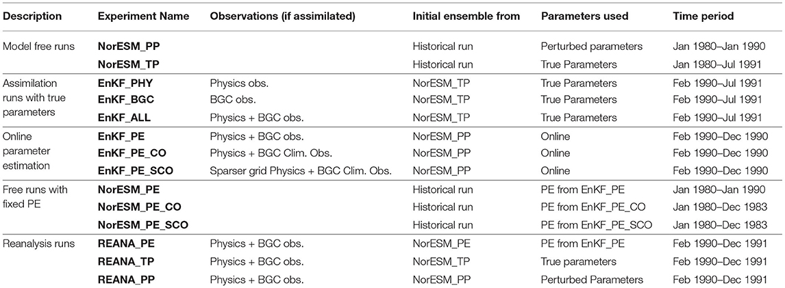
Table 1. List of performed experiments.
3. Results
3.1. Impact of Assimilation on the State Using True Parameters
A prerequisite for skillful parameter estimation is that assimilation constrains the error of the state variables well. Error in state variables, particularly at the surface and at inter-mediate depth can have a strong influence on near-surface biogeochemical processes. We work in a perfect model framework (i.e., all members use true parameter values) and we are interested in how well the error of the state variables is constrained by different observation networks. The monthly time evolution of the RMSE (averaged over the global domain and organized by depth level) of the NorESM free ensemble run (NorESM_TP) is shown in Figures 2, 3. We also show the RMSE-difference (RMSED) of EnKF_PHY, EnKF_BGC and EnKF_ALL assimilation experiments compared to NorESM_TP.
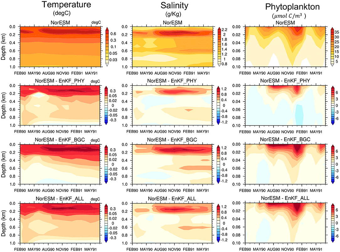
Figure 2. The first row shows the time evolution of the vertical global-averaged RMSE for temperature (first column), salinity (second column), and phytoplankton concentration (third column) in the NorESM free run against TRUTH. The other rows show the RMSE difference (RMSED) for the same variables with assimilation of physics observation (EnKF_PHY), BGC surface observations (EnKF_BGC), and combined observations (EnKF_ALL), respectively. RMSED is computed by subtracting the RMSE of simulations with DA from that of free run RMSE. Warm (cold) colors represent improvement (degradation) from assimilation.
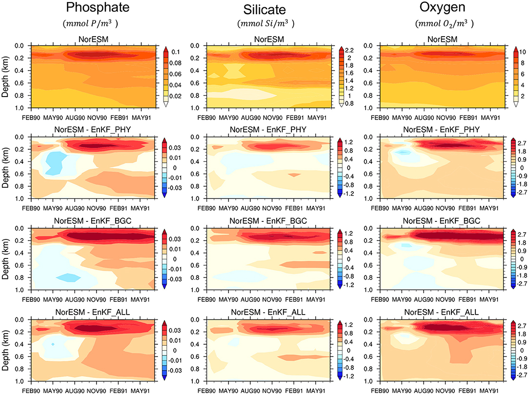
Figure 3. Same as Figure 2 but for Phosphate (first column), Silicate (second column), and Oxygen (third column).
All assimilation experiments improve the accuracy of both the ocean and the BGC state variables in the near-surface levels compared to NorESM_TP. The difference between the three DA experiments is small. Sole assimilation of BGC or physical data alone is able to constrain well the surface ocean physical and biogeochemical variables and vice versa. This was somewhat unexpected, and it exemplifies well the potential of strongly coupled data assimilation (Penny and Hamill, 2017). It should be reminded that we assimilate in an isopycnal coordinate that has been shown to be more effective than assimilation in geopotential depth for surface observation (Gavart and De Mey, 1997; Counillon et al., 2016). The Analysis error for phytoplankton concentration is well reduced in all experiments. Similarly, clear improvements are shown for nutrients (phosphate and silicate) and oxygen estimates. BGC data assimilation alone yields the largest reduction of errors in the top 200 m. Below 200 m depth, the combined assimilation of physical and BGC observations provides slightly better performance than the other two experiments and it mitigates the degradation seen at deeper layers for some variables, e.g., temperature, phosphate, and oxygen. Overall, the accuracy of the combined assimilation experiment is slightly better. For example, the average error in EnKF_ALL for salinity in the top 1 km is 35% lower than that of the free run, while it is 24% for EnKF_PHY and 30% for EnKF_BGC. Similarly for Oxygen, EnKF_ALL has 28% lower error than the free run while EnKF_PHY is 19% and EnKF_BGC 24%.
3.2. Online Parameter Estimation
This section presents and assesses spatially varying ecosystem parameters estimation with the DOSA scheme (reduction of error of the estimated parameter). We analyse the EnKF_PE, EnKF_PE_CO and EnKF_PE_SCO experiments (see Table 1). The time evolution of the global-averaged ensemble spreads and RMSEs of the estimated parameters obtained from EnKF_PE are shown in Figure 4. RMSEs for all parameters reduce with time and become stable within one year of assimilation. The reduction is largest for GRAZRA that shows a 72% error reduction from its initial distribution (Table 2). The error reduction in the remaining parameters WPOC, BKPHY, GAMMAP, and BKOPAL is about 54, 47, 40, and 30%, respectively. Similarly, the ensemble spreads of all parameters reduce with time. However, the reduction is quicker than for RMSE, which suggests that the system may benefit from using multiplicative or additive inflation (Mitchell and Houtekamer, 2000; Anderson, 2001). Similar results have been obtained from EnKF_PE_CO and EnKF_PE_SCO experiments (not shown).
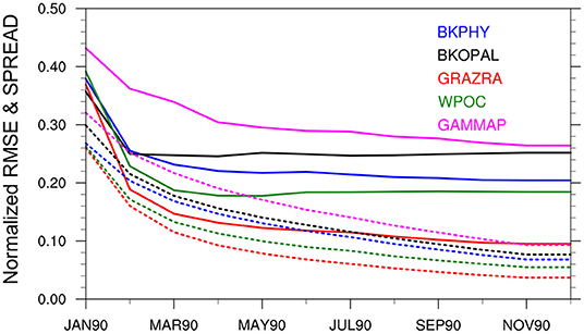
Figure 4. Time evolution of global-averaged normalized RMSE (solid lines) and ensemble spread (dotted lines) of the BGC parameters from state-parameter estimation experiment using assimilation of time-varying observations (EnKF_PE). RMSE is calculated by comparing each member against the true values. Both RMSE and spread has been normalized by the global mean value of the true parameter.
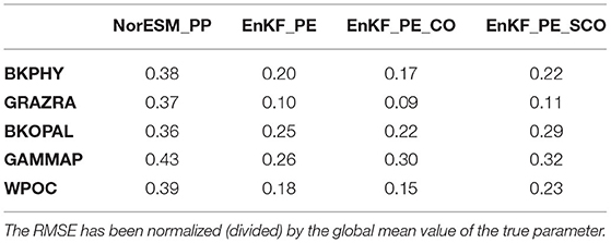
Table 2. Spatial average of the point-wise ensemble RMSE of the parameter values obtained at the end of the estimation period (December 1990).
Ensemble data assimilation estimates the parameters based on their correlation with the model misfits from observations (e.g., Anderson, 2001). In order to visualise the convergence process, we have used scatter plots (see Figure 5) of the parameter ensemble against the model deviation from the truth at different cycles of the assimilation experiment; i.e., in the start in January 1990 (red color), after the first assimilation, the second and the last assimilation cycles (green, purple, and blue colors, respectively). Each scattered dot represents one ensemble member and the big dots represent the ensemble mean. All ecosystem variables simulated using perturbed parameters show relatively large deviations from the TRUTH (y-axes in Figure 5), which underlines the sensitivity of the surface quantities to errors in the parameters. Among all parameters, GRAZRA shows the strongest linear relation with all variables and is the most important parameter for reducing model bias. For some parameters, the linear relationship is only strong with respect to some variables (e.g., WPOC with Silicate), which shows the importance of using multiple type of observations for the parameter estimation. The parameters are converging toward the true value very rapidly (already within the first 2 assimilation cycles), strongly reducing the error in ecosystem variables. After 11 assimilation cycles (corresponding to December 1990), one can notice that global means of the estimated parameters are very close to the true value and that the errors in the ecosystem variables are close to zero. This shows that the method converges quickly (within few assimilation steps) and is able to constrain the global mean of estimated parameters close to their true values by largely reducing the error in parameters. Similar results have been found for EnKF_PE_CO and EnKF_PE_SCO experiments (not shown).
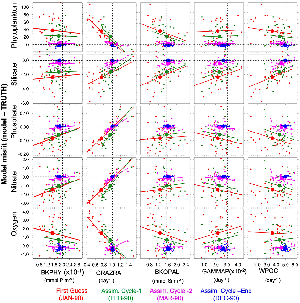
Figure 5. Scatter plots for globally-averaged misfit (model-TRUTH) ensemble vs. BGC parameters ensemble. Plots are shown for surface phytoplankton (row-one), silicate (row-two), phosphate (row-three), nitrate (row-four), and oxygen (row-five) with BKPHY (column-one), GRAZRA, (column-two), BKOPAL (column-three), GAMMAP (column-four), and WPOC (column-five) parameters; obtained from first guess (red), after first assimilation cycle (green), second assimilation cycle (purple), and end of assimilation (blue) with EnKF_PE experiment. The large dots show the ensemble mean. Horizontal and vertical dashed black reference lines represent the line of zero misfit and global-averaged TP values, respectively. Solid colored lines are the linear regression lines.
We further analyse the spatial distribution of the estimated parameters obtained for December 1990 from all three experiments. Figure 6 shows the true and ensemble mean of the experiments with perturbed and estimated parameters. First, we note that the data assimilation yields a reduction of error compared to the initial values for all parameters. We can also notice that there is some spatial coherency in the value of the pattern retrieved. Parameters show relatively good agreement with the spatial distribution of the true value with spatial RMSE reduced by 75% for GRAZRA, by 50 % for BKPHY and WPOC, 40% for GAMMAP, and only 30% for BKOPAL, see Table 2. However, some differences remain and there is some small-scale noise. We suspect the latter to be related to spurious correlations present in our finite size ensemble (30). The places where the estimation fails to converge to true value may relate to places where the model is insensitive to the parameters. Hence, the parameter estimation can drift towards an erroneous value—e.g., as a response to spurious correlation or because of the approximation of Gaussianity and linearity during the analysis—without having an impact on the state error. In order to assess the impact of the error reduction on the state variable, we will freeze the parameter values at the last assimilation cycle and perform simulations in a free ensemble run and in a reanalysis mode in the following sections.
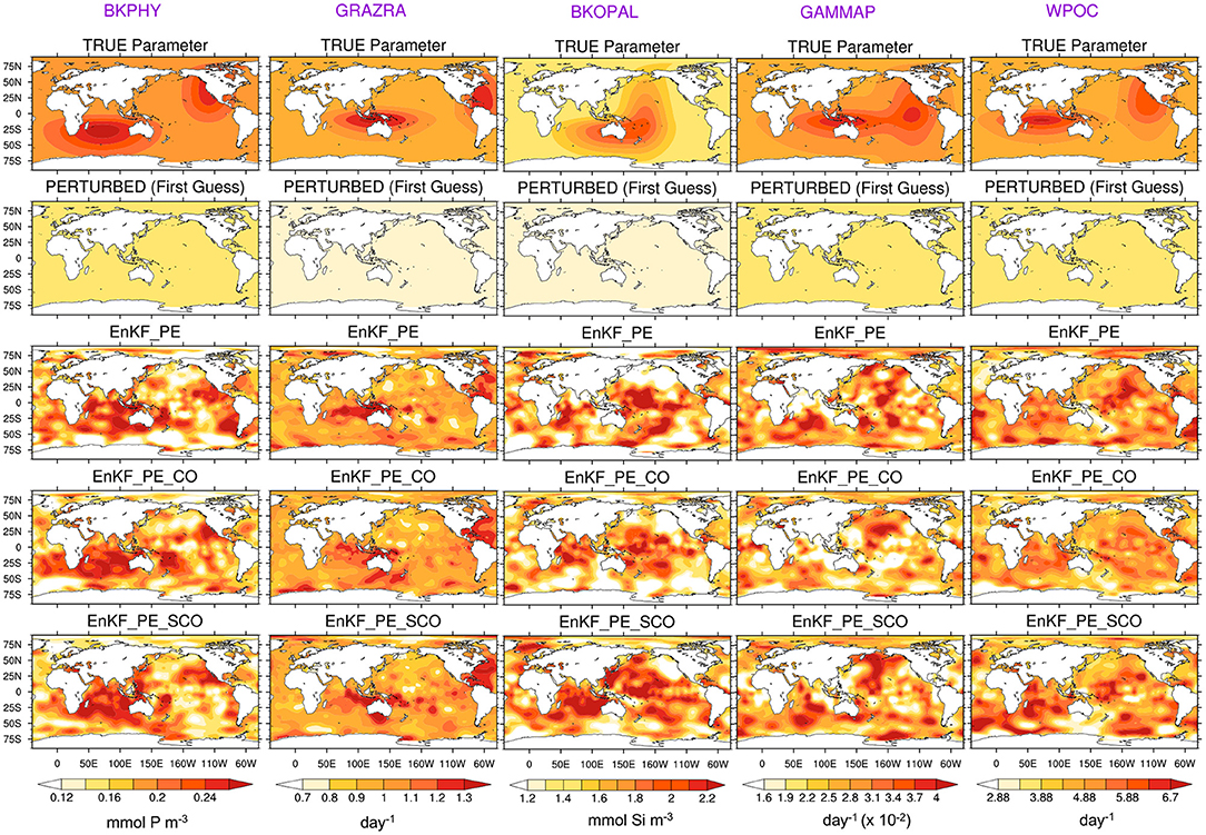
Figure 6. True (row-one) and point wise ensemble mean of the perturbed (row-two) and estimated BGC parameters in December 1990 with assimilation of time-varying (row-three), climatological (row-four), and very sparse climatological (row-five) BGC surface observations in addition to time varying physics. Column-one to -five correspond to BKPHY, GRAZRA, BKOPAL, GAMMAP, and WPOC parameters.
3.3. Model Ensemble Free Run With Estimated Parameters
We verify the state accuracy of a free ensemble run that uses the final parameter's estimates of EnKF_PE, EnKF_PE_CO and EnKF_PE_SCO experiments, and refer to them as NorESM_PE, NorESM_PE_CO and NorESM_PE_SCO, respectively. We compare the performance against a free ensemble run using the true parameter (NorESM_TP) and one using the perturbed parameter (NorESM_PP).
In Figure 7, NorESM_PP poorly simulates the phytoplankton activity with a systematic overestimation of phytoplankton concentrations and generally longer spring blooms during the summer seasons compared to NorESM_TP. The runs that use the estimated parameters clearly outperform NorESM_PP, and perform closely to NorESM_TP. For instance, the global averaged RMSE of the phytoplankton concentration with NorESM_PE and NorESM_TP is roughly 51 and 54% lower than in NorESM_PP. Similarly, the biases in the parameter estimation experiments are significantly reduced to the level of that of TP. The performance of TP and PEs are also comparable in the upper 200-m as shown in Figure 7C. Below this depth, the model seems to have no sensitivity to these parameters and all experiments perform equivalently.
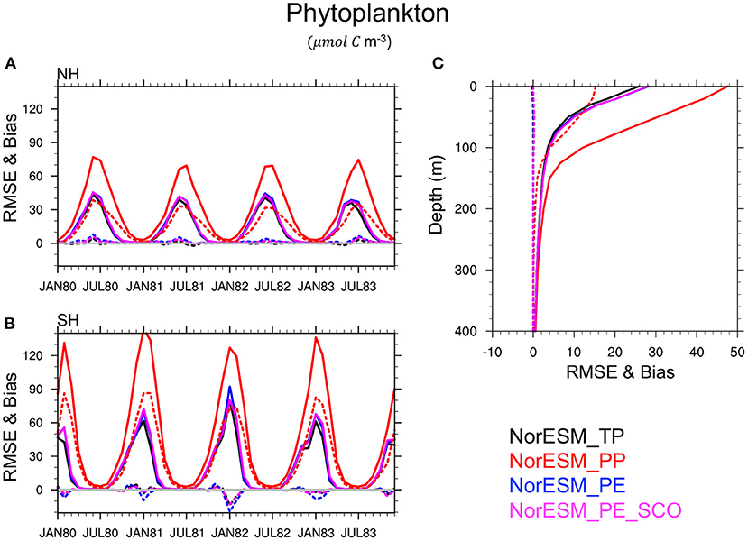
Figure 7. Panels on the left show the RMSE (solid lines) and bias (dotted lines) of the ensemble mean of NorESM phytoplankton concentration compared to the TRUTH in the euphotic zone (i.e., from the surface to 100 m) in the northern hemisphere [NH, (A)] and in the southern hemisphere [SH, (B)]. (C) is the globally averaged vertical error profiles estimated over the 4-year period (1980–1983). The results of the free NorESM simulation using TP are shown in black, PP in red, and PE using assimilation of time-varying observations in blue and sparse climatological BGC observations in magenta.
This conclusion is also verified for others BGC quantities such as silicate (Figure 8), phosphate (Figure 9), nitrate, and oxygen (not shown) in which PEs perform nearly as good as TP, while PP leads to a poor simulation of these variables and a large underestimate (negative bias) of the nutrient concentration, specifically during summer seasons, in the euphotic zone. This is related to the highly enhanced phytoplankton activity in PP, as seen earlier, which removes the available nutrients from the euphotic zone. RMSE and bias profile plots suggest that BGC parameters may strongly control the biogeochemical process in deeper layers up to roughly 500 m depth. Again, the simulated quality of nutrients and oxygen profiles by PEs and TP are very similar throughout entire depth.
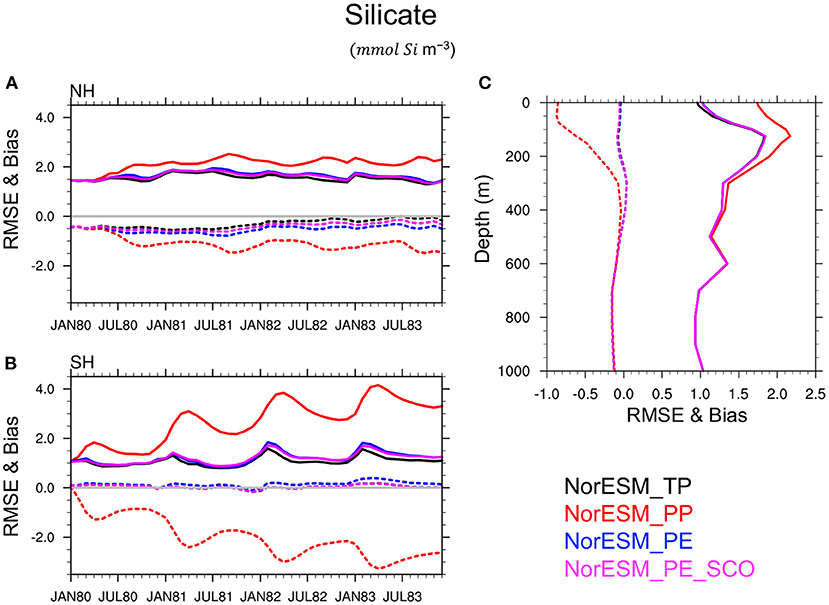
Figure 8. Same as Figure 7 but for Silicate.
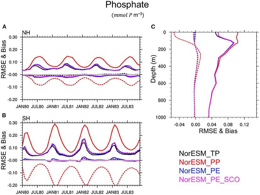
Figure 9. Same as Figure 7 but for Phosphate.
We can also notice that NorESM_PE and NorESM_PE_SCO experiments show very comparable accuracy for ecosystem variables. Results from NorESM_PE_CO is not included to avoid overlapping lines in the Figures but we found very similar results. It suggests that BGC surface sparse climatological observations, and even very sparse climatological observations are somewhat sufficient to retrieve optimal ecosystem parameters with similar quality as time-varying observations using the DOSA-EnKF algorithm. Hence, in our model, the largest contribution to the error appears to be related to the seasonal cycle representation, which can be effectively corrected with a monthly climatology of observations.
We also analyse the impact of the parameters spatially. Figure 10 shows the RMSE and bias averaged over 100 m depth for the phytoplankton concentration and 500 m for the silicate profile. In general, bloom intensity increases from mid to high latitudes. It is seen that PP shows a larger overestimation of phytoplankton concentration, specifically over high latitudes and over some tropical regions, e.g., the eastern tropical Pacific Ocean. In all 3 PEs, the biases and RMSEs are reduced. The RMSE and bias patterns of the PEs closely match that of TP. In the case of silicate, PP shows a severe underestimation over the region where increased phytoplankton activities are seen.
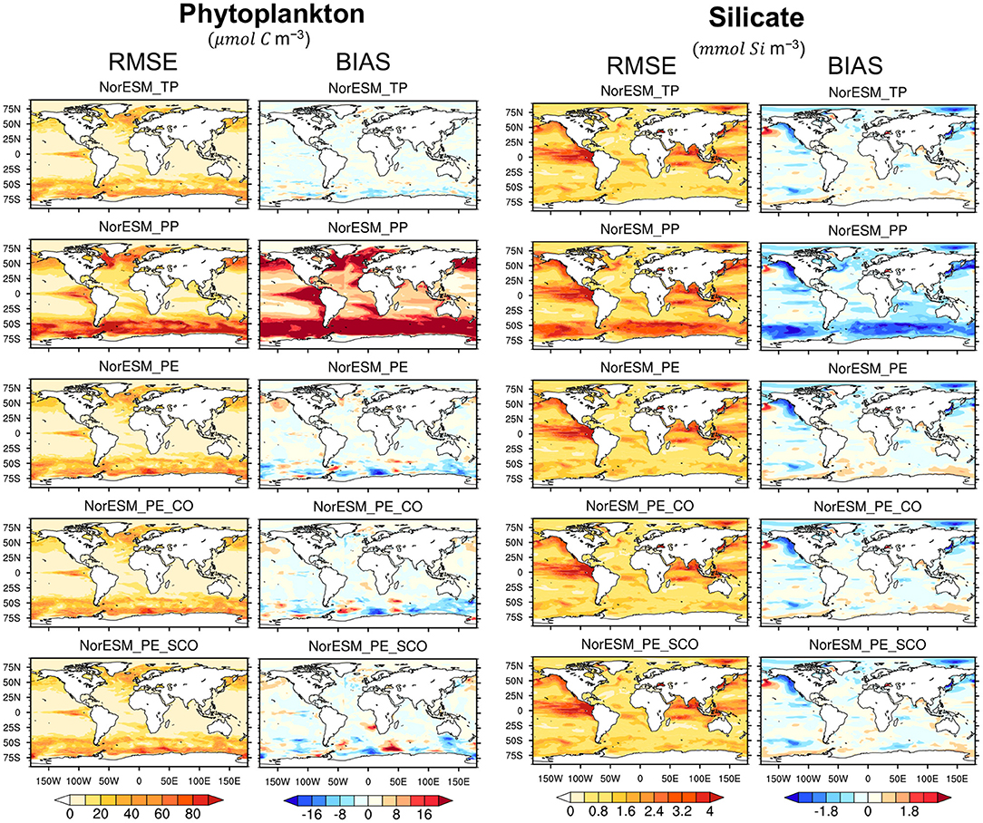
Figure 10. RMSE and bias maps estimated over 1980–1983 for phytoplankton and silicate. For phytoplankton, RMSE (column-one) and bias (column-two) are averaged over euphotic zone (0–100 m), while for silicate, they are averaged over 0–500 m depth (column-three and -four, respectively). The error are computed from free NorESM simulation using TP (first row), PP (row-two), and fixed PE estimated with assimilation of time-varying observation (row-three), time varying physic and climatological BGC (row-four), and time varying physic and sparse climatological BGC (row-five).
Performance of the PEs is now assessed for an observation that was not used for tuning the parameters. Hence, we investigate air-sea CO2 flux and net primary production (NPP) (Figure 11) and found consistent results. Similar to previous results, PEs maintain the accuracy closer to TP.

Figure 11. Same as Figure 10 but for CO2 flux (column-one and -two) and net primary production (column-three and -four).
The above results provide strong evidence that the DOSA-EnKF system can successfully recover the optimal value for chosen BGC parameters. It also suggests that the remaining parametric error does not effectively influence the behavior of the model.
3.4. Reanalysis With Estimated Parameters
This section presents the accuracy of the state variables in the reanalyses which started in February 1990 and were run until December 1991 using fixed estimated parameters (REANA_PE). We compare the performance of REANA_PE with that of a reanalysis using perturbed parameters REANA_PP (lower benchmark) and a reanalysis using true parameters REANA_TP (upper benchmark).
The time evolution of the RMSE and bias over the euphotic zone is presented in Figure 12. First, we notice that assimilation improves the accuracy of the ecosystem variables in all experiments. For instance, the prior distributions of phytoplankton, oxygen and net primary production (NPP) are associated with high uncertainty and biases in the months with maximum bloom activity (January in the southern hemisphere). After a few assimilation cycles, there is a lower error during the bloom seasons. This can also be verified by comparing the phytoplankton free run accuracy shown in Figure 7 with the analysis accuracy presented here. For instance, the free run with PP shows RMSE values of roughly 70 μmolC m−3 for the spring bloom peak over the northern hemisphere (Figure 7), which is reduced to roughly 40 μmolC m−3 after assimilation (Figure 12).
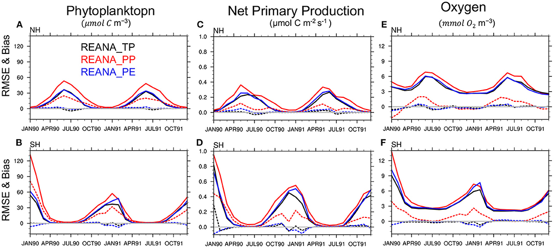
Figure 12. Panels on the left show the RMSE (solid lines) and bias (dotted lines) of the ensemble mean of phytoplankton concentration reanalysis compared to the TRUTH in the euphotic zone in the northern hemisphere [NH, (A)] and southern hemisphere [SH, (B)]. The results of the reanalysis using TP are shown in black, PP in red, and PE in blue using assimilation of time-varying observations. (C,D) and (E,F) are same as (A,B) but for net primary production and oxygen concentration.
Similar results are found for NPP (time evolution of free run not shown), for which observations are not being assimilated in the system (non-observed variable). Thus, the assimilation system is capable of improving the quality of not only the observed ecosystem variables (e.g., phytoplankton and Oxygen) but also of the non-observed variables. However, differences in the accuracy of reanalyses are clearly visible for the different set of parameters. REANA_PP shows larger uncertainty and stronger biases particularly during bloom seasons for phytoplankton, oxygen and net primary production reanalyses. The differences between REANA_PP and REANA_TP are more pronounced in the northern hemisphere than in the southern hemisphere. This exemplifies that assimilation cannot achieve optimum performance in the presence of model error.
The quality assessment of reanalysis has been further assessed in the deeper ocean by estimating the globally averaged RMSE and bias profiles for the top 1-km (Figure 13). The statistics have been computed using the July 1990 to December 1991 period. The first 6 months have been discarded for removing assimilation spinup that is longer in the deeper ocean. TP and PE show overall comparable performance for phytoplankton reanalysis whereas PP leads to degraded performance mostly in the top 150 m. Similar results can be seen for nutrients (e.g., phosphate and silicate) and oxygen profiles where differences of PP with TP or PE are more pronounced at inter-mediate depth levels. Still we can see that the performance of PE is not as efficient for oxygen and phosphate below 300 m. It would have been interesting to test whether training the parameters with deeper BGC observations (currently only available at the surface) would have improved performance there.

Figure 13. (A) is the globally averaged RMSE (solid lines) and bias (dotted lines) profiles estimated over the 18-months reanalysis period (July 1990- December 1991) for phytoplankton concentration generated using TP (black), PP (red), fixed PE (blue), and assimilating time-varying observations. (B–D) are same as (A) but for oxygen, phosphate, and silicate, respectively.
4. Summary and Conclusions
We have presented the feasibility of optimizing spatially varying ocean biogeochemical parameters in an Earth system model using an ensemble-based data assimilation method in an idealized perfect twin experiment setup. We used the NorCPM system, which combines the NorESM global model with the DOSA-EnKF assimilation method. The DOSA-EnKF applies a smoothing step to the state and parameters before propagating the model for the analysis step. We estimate five spatially varying biogeochemical parameters in addition to ocean physical and biogeochemical state variables. The parameters characterize the major surface biological processes such as phytoplankton growth, zooplankton grazing, release of dissolved organic carbon, sinking of organic matter and nutrient uptake. We assimilate synthetic monthly ocean physics profiles (temperature and salinity) and surface BGC observations (Phytoplankton, Nitrate, Phosphate, Silicate, and Oxygen) in a strongly coupled framework, where observations are used to update ocean and BGC state variables jointly along with parameters.
Assimilation of different observation networks in a strongly coupled framework reveals that BGC observations can effectively constrain errors in the ocean physics and vice versa. It demonstrates the potential of strongly coupled data assimilation to constrain the errors in cross component state variables. It could benefit ocean BGC in real observations setup, where dense network of physical observations can be used to constrain the BGC state variables for which measured properties are under-sampled. In our setup, sole assimilation of BGC surface observations seems to yield largest error reduction in the top 200 m for both physical and ecosystem variables. Further, combined assimilation of physical and BGC observations provides more robust performance and avoid degradation in deeper layers.
The success of the parameter estimation has been tested by three state-parameter estimation experiments performed using different networks of BGC observation on top of physical observations. One of them assimilating sparse-grid (every 5th grid cell) time-varying BGC observations and the other two assimilating climatological BGC observations prepared at sparse (every 5th grid cell) and very sparse horizontal resolution (every 10th grid cell). All experiments converge quickly within a year and are able to retrieve the true global mean of estimated parameters, strongly reducing the error in the perturbed parameters. Further, the spatial pattern for nutrient uptake and zooplankton grazing parameters show relatively good agreement with that of the true values. However, some differences remain in the estimated values. The success of recovering the true parameter values in any region depends on the sensitivity of the model to those parameters. It is possible that the true values are not sensitive in many regions. Over such regions, the estimation of parameters may not work effectively and differences between estimated and true values are possible.
As a way to test the impact of the parameters on the state variables, we conducted ensemble free run using estimated parameter values obtained from three different BGC observation networks mentioned earlier. The performance of the estimated values has been compared with upper- and lower benchmark model ensemble runs conducted using true and perturbed parameter values, respectively. We found that the accuracy of simulated ecosystem variables obtained using all three sets of estimated parameters is as good as those obtained using true parameters. Perturbed parameters lead to a systematic overestimation of the phytoplankton and longer spring blooms compared to the true parameters. Similar results have been obtained for nutrient and oxygen concentrations throughout the entire water column. These results suggest that remaining differences in the estimated and true parameters do not effectively influence the behavior of the model and estimated values are optimal. As similar results have been obtained from all three sets of estimated parameters, we can conclude that very sparse BGC surface climate observations are sufficient to retrieve optimal ecosystem parameters with similar quality as time-varying observations using the DOSA-EnKF algorithm with our model system. We suspect that this is because the primary source of error is in the representation of the seasonal cycle that is well represented by the monthly climatology data.
The performance of reanalyses using fixed estimated parameters was also assessed. Again, we found that using the estimated parameters improves the quality of ecosystem variables in the reanalyses mode. The accuracy of the reanalysis with perturbed parameters shows poorer performance than the one using true and estimated parameters with large biases and error for observed variables (e.g., phytoplankton, oxygen and phosphate) as well as for unobserved variables (e.g., net primary production which was not assimilated). This is expected because assimilation is not designed to correct model errors (Dee, 2005; Counillon et al., 2021).
The finding of this study clearly reveals that the DOSA-EnKF system in a perfect twin experiment can estimate spatially varying optimal BGC parameters for the NorESM model, even with very sparse climatological BGC surface observation. It remains to be confirmed whether the method succeeds in a real framework (assimilating real observations) as errors may originate from the other components (atmosphere, ocean physics, sea ice) or additional structural-related errors.
Data Availability Statement
The raw data supporting the conclusions of this article will be made available by the authors, without undue reservation.
Author Contributions
TS, FC, JT, and MG contributed to conception and design of the study. TS performed the numerical experiments and the statistical analysis. TS and FC wrote the first draft of the manuscript. JT, YW, and MG wrote sections of the manuscript. All authors contributed to manuscript revision, read, and approved the submitted version.
Funding
This study was partly funded by the Centre for climate dynamics at the Bjerknes Centre and the Research Council of Norway (INES; grant no. 270061). This work has also received funding from (EU Horizon 2020 Framework Programme) EU-TRIATLAS (grant no. 817578) and from the Trond Mohn stiftelse (grant no. BFS2018TMT01). This work has also received a grant for computer time from the Norwegian Program for supercomputing (NOTUR2, project number nn9039k) and a storage grant (NORSTORE, NS9039k). JT acknowledges funding from Research Council of Norway (COLUMBIA; grant no. 275268). YW acknowledges support from the Research Council of Norway under the CoRea project (grant no. 301396).
Conflict of Interest
The authors declare that the research was conducted in the absence of any commercial or financial relationships that could be construed as a potential conflict of interest.
Publisher's Note
All claims expressed in this article are solely those of the authors and do not necessarily represent those of their affiliated organizations, or those of the publisher, the editors and the reviewers. Any product that may be evaluated in this article, or claim that may be made by its manufacturer, is not guaranteed or endorsed by the publisher.
References
Ait-El-Fquih, B., Gharamti, M. E., and Hoteit, I. (2016). A bayesian consistent dual ensemble kalman filter for state-parameter estimation in subsurface hydrology. Hydrol. Earth Syst. Sci. 20, 3289–3307. doi: 10.5194/hess-20-3289-2016
Anav, A., Friedlingstein, P., Kidston, M., Bopp, L., Ciais, P., Cox, P., et al. (2013). Evaluating the land and ocean components of the global carbon cycle in the cmip5 earth system models. J. Clim. 26, 6801–6843. doi: 10.1175/JCLI-D-12-00417.1
Anderson, J. L. (2001). An ensemble adjustment kalman filter for data assimilation. Month. Weather Rev. 129, 2884–2903. doi: 10.1175/1520-0493(2001)129<2884:AEAKFF>2.0.CO;2
Annan, J., Hargreaves, J., Edwards, N., and Marsh, R. (2005). Parameter estimation in an intermediate complexity earth system model using an ensemble kalman filter. Ocean Model. 8, 135–154. doi: 10.1016/j.ocemod.2003.12.004
Arnold Jr, C. P., and Dey, C. H. (1986). Observing-systems simulation experiments: past, present, and future. Bull. Amer. Meteorol. Soc. 67, 687–695. doi: 10.1175/1520-0477(1986)067<0687:OSSEPP>2.0.CO;2
Assmann, K., Bentsen, M., Segschneider, J., and Heinze, C. (2010). An isopycnic ocean carbon cycle model. Geosci. Model Dev. 3, 143–167. doi: 10.5194/gmd-3-143-2010
Bellenger, H., Guilyardi, É., Leloup, J., Lengaigne, M., and Vialard, J. (2014). Enso representation in climate models: from cmip3 to cmip5. Clim. Dyn. 42, 1999–2018. doi: 10.1007/s00382-013-1783-z
Bentsen, M., Bethke, I., Debernard, J., Iversen, T., Kirkevåg, A., Seland, Ø., et al. (2012). The norwegian earth system model, noresm1-m–part 1: description and basic evaluation. Geosci. Model Dev. Discuss. 5, 2843–2931. doi: 10.5194/gmdd-5-2843-2012
Bentsen, M., Bethke, I., Debernard, J. B., Iversen, T., Kirkevåg, A., Seland, Ø., et al. (2013). The norwegian earth system model, noresm1-m–part 1: description and basic evaluation of the physical climate. Geosci. Model Dev. 6, 687–720. doi: 10.5194/gmd-6-687-2013
Bertino, L., Evensen, G., and Wackernagel, H. (2003). Sequential data assimilation techniques in oceanography. Int. Stat. Rev. 71, 223–241. doi: 10.1111/j.1751-5823.2003.tb00194.x
Bethke, I., Wang, Y., Counillon, F., Keenlyside, N., Kimmritz, M., Fransner, F., et al. (2021). Norcpm1 and its contribution to cmip6 dcpp. Geosci. Model Dev. Discuss. 14, 1–84. doi: 10.5194/gmd-14-7073-2021
Bleck, R., Rooth, C., Hu, D., and Smith, L. T. (1992). Salinity-driven thermocline transients in a wind-and thermohaline-forced isopycnic coordinate model of the north atlantic. J. Phys. Oceanograph. 22, 1486–1505.
Bleck, R., and Smith, L. T. (1990). A wind-driven isopycnic coordinate model of the north and equatorial atlantic ocean: 1. model development and supporting experiments. J. Geophys. Res. Oceans 95, 3273–3285.
Bopp, L., Resplandy, L., Orr, J. C., Doney, S. C., Dunne, J. P., Gehlen, M., et al. (2013). Multiple stressors of ocean ecosystems in the 21st century: projections with cmip5 models. Biogeosciences 10, 6225–6245. doi: 10.5194/bg-10-6225-2013
Chen, Y., and Zhang, D. (2006). Data assimilation for transient flow in geologic formations via ensemble kalman filter. Adv. Water Resour. 29, 1107–1122. doi: 10.1016/j.advwatres.2005.09.007
Counillon, F., Bethke, I., Keenlyside, N., Bentsen, M., Bertino, L., and Zheng, F. (2014). Seasonal-to-decadal predictions with the ensemble kalman filter and the norwegian earth system model: a twin experiment. Tellus Dyn. Meteorol. Oceanograph. 66:21074. doi: 10.3402/tellusa.v66.21074
Counillon, F., Keenlyside, N., Bethke, I., Wang, Y., Billeau, S., Shen, M. L., and Bentsen, M. (2016). Flow-dependent assimilation of sea surface temperature in isopycnal coordinates with the norwegian climate prediction model. Tellus Dyn. Meteorol. Oceanograph. 68:32437. doi: 10.3402/tellusa.v68.32437
Counillon, F., Keenlyside, N., Toniazzo, T., Koseki, S., Demissie, T., Bethke, I., and Wang, Y. (2021). Relating model bias and prediction skill in the equatorial atlantic. Clim. Dyn. 56, 2617–2630. doi: 10.1007/s00382-020-05605-8
Craig, A. P., Vertenstein, M., and Jacob, R. (2012). A new flexible coupler for earth system modeling developed for ccsm4 and cesm1. Int. J. High Perform. Comput. Appl. 26, 31–42. doi: 10.1177/1094342011428141
Dee, D. P. (2005). Bias and data assimilation. Quart. J. R. Meteorol. Soc. J. Atmosph. Sci. Appl. Meteorol. Phys. Oceanography 131, 3323–3343. doi: 10.1256/qj.05.137
Doron, M., Brasseur, P., Brankart, J.-M., Losa, S. N., and Melet, A. (2013). Stochastic estimation of biogeochemical parameters from globcolour ocean colour satellite data in a north atlantic 3d ocean coupled physical–biogeochemical model. J. Marine Syst. 117, 81–95. doi: 10.1016/j.jmarsys.2013.02.007
Eknes, M., and Evensen, G. (2002). An ensemble kalman filter with a 1-d marine ecosystem model. J. Marine Syst. 36, 75–100. doi: 10.1016/S0924-7963(02)00134-3
Evensen, G. (2003). The ensemble kalman filter: theoretical formulation and practical implementation. Ocean Dyn. 53, 343–367. doi: 10.1007/s10236-003-0036-9
Fransner, F., Counillon, F., Bethke, I., Tjiputra, J., Samuelsen, A., Nummelin, A., et al. (2020). Ocean biogeochemical predictions–initialization and limits of predictability. Front. Marine Sci. 7:386. doi: 10.3389/fmars.2020.00386
Gaspari, G., and Cohn, S. E. (1999). Construction of correlation functions in two and three dimensions. Quart. J. R. Meteorol. Soc. 125, 723–757.
Gavart, M., and De Mey, P. (1997). Isopycnal eofs in the azores current region: a statistical tool fordynamical analysis and data assimilation. J. Phys. Oceanography 27, 2146–2157.
Gent, P. R., Danabasoglu, G., Donner, L. J., Holland, M. M., Hunke, E. C., Jayne, S. R., et al. (2011). The community climate system model version 4. J. Clim. 24, 4973–4991. doi: 10.1175/2011JCLI4083.1
Gharamti, M., Ait-El-Fquih, B., and Hoteit, I. (2015). An iterative ensemble kalman filter with one-step-ahead smoothing for state-parameters estimation of contaminant transport models. J. Hydrol. 527, 442–457. doi: 10.1016/j.jhydrol.2015.05.004
Gharamti, M., Samuelsen, A., Bertino, L., Simon, E., Korosov, A., and Daewel, U. (2017a). Online tuning of ocean biogeochemical model parameters using ensemble estimation techniques: application to a one-dimensional model in the north atlantic. J. Marine Syst. 168, 1–16. doi: 10.1016/j.jmarsys.2016.12.003
Gharamti, M., Tjiputra, J., Bethke, I., Samuelsen, A., Skjelvan, I., Bentsen, M., et al. (2017b). Ensemble data assimilation for ocean biogeochemical state and parameter estimation at different sites. Ocean Model. 112, 65–89. doi: 10.1016/j.ocemod.2017.02.006
Goris, N., Tjiputra, J. F., Olsen, A., Schwinger, J., Lauvset, S. K., and Jeansson, E. (2018). Constraining projection-based estimates of the future north atlantic carbon uptake. J. Clim. 31, 3959–3978. doi: 10.1175/JCLI-D-17-0564.1
Halem, M., and Dlouhy, R. (1984). “Observing system simulation experiments related to space-borne lidar wind profiling. part 1: forecast impacts of highly idealized observing systems,” in Conference on Satellite Meteorology/Remote Sensing and Applications (Clearwater, FL: American Meteorological Society), 272–279.
Halliwell Jr, G., Srinivasan, A., Kourafalou, V., Yang, H., Willey, D., Le Hénaff, M., et al. (2014). Rigorous evaluation of a fraternal twin ocean osse system for the open gulf of mexico. J. Atmosph. Ocean. Technol. 31, 105–130. doi: 10.1175/JTECH-D-13-00011.1
Holland, M. M., Bailey, D. A., Briegleb, B. P., Light, B., and Hunke, E. (2012). Improved sea ice shortwave radiation physics in ccsm4: the impact of melt ponds and aerosols on arctic sea ice. J. Clim. 25, 1413–1430. doi: 10.1175/JCLI-D-11-00078.1
Houtekamer, P. L., and Mitchell, H. L. (2001). A sequential ensemble kalman filter for atmospheric data assimilation. Month. Weather Rev. 129, 123–137. doi: 10.1175/1520-0493(2001)129<0123:ASEKFF>2.0.CO;2
Jazwinski, A. H. (2007). Stochastic Processes and Filtering Theory. Mineola, NY: Dover Publications.
Jochum, M., Yeager, S., Lindsay, K., Moore, K., and Murtugudde, R. (2010). Quantification of the feedback between phytoplankton and enso in the community climate system model. J. Clim. 23, 2916–2925. doi: 10.1175/2010JCLI3254.1
Keenlyside, N., Latif, M., Jungclaus, J., Kornblueh, L., and Roeckner, E. (2008). Advancing decadal-scale climate prediction in the north atlantic sector. Nature 453, 84–88. doi: 10.1038/nature06921
Kessler, A., and Tjiputra, J. (2016). The southern ocean as a constraint to reduce uncertainty in future ocean carbon sinks. Earth Syst. Dyn. 7, 295–312. doi: 10.5194/esd-7-295-2016
Kimmritz, M., Counillon, F., Smedsrud, L. H., Bethke, I., Keenlyside, N., Ogawa, F., et al. (2019). Impact of ocean and sea ice initialisation on seasonal prediction skill in the arctic. J. Adv. Model. Earth Syst. 11, 4147–4166. doi: 10.1029/2019MS001825
Kirkevåg, A., Iversen, T., Seland, Ø., Hoose, C., Kristjánsson, J., Struthers, H., et al. (2013). Aerosol–climate interactions in the norwegian earth system model–noresm1-m. Geosci. Model Dev. 6, 207–244. doi: 10.5194/gmd-6-207-2013
Kwiatkowski, L., Torres, O., Bopp, L., Aumont, O., Chamberlain, M., Christian, J. R., et al. (2020). Twenty-first century ocean warming, acidification, deoxygenation, and upper-ocean nutrient and primary production decline from cmip6 model projections. Biogeosciences 17, 3439–3470. doi: 10.5194/bg-17-3439-2020
Lawrence, D. M., Oleson, K. W., Flanner, M. G., Thornton, P. E., Swenson, S. C., Lawrence, P. J., et al. (2011). Parameterization improvements and functional and structural advances in version 4 of the community land model. J. Adv. Model. Earth Syst. 3:M03001. doi: 10.1029/2011MS00045
Losa, S. N., Kivman, G. A., and Ryabchenko, V. A. (2004). Weak constraint parameter estimation for a simple ocean ecosystem model: what can we learn about the model and data? J. Marine Syst. 45, 1–20. doi: 10.1016/j.jmarsys.2003.08.005
Losa, S. N., Kivman, G. A., Schröter, J., and Wenzel, M. (2003). Sequential weak constraint parameter estimation in an ecosystem model. J. Marine Syst. 43, 31–49. doi: 10.1016/j.jmarsys.2003.06.001
Lovenduski, N. S., Yeager, S. G., Lindsay, K., and Long, M. C. (2019). Predicting near-term variability in ocean carbon uptake. Earth Syst. Dyn. 10, 45–57. doi: 10.5194/esd-10-45-2019
Maier-Reimer, E., Kriest, I., Segschneider, J., and Wetzel, P. (2005). The hamburg ocean carbon cycle model HAMOCC 5.1 (2005). Technical description release 1.1, Reports on Earth System Science. Hamburg: Max Planck Institute for Meteorology. Available online at: https://mpimet.mpg.de/fileadmin/publikationen/erdsystem_14.pdf
Marotzke, J., Jakob, C., Bony, S., Dirmeyer, P. A., O'Gorman, P. A., Hawkins, E., et al. (2017). Climate research must sharpen its view. Nat. Clim. Change 7, 89–91. doi: 10.1038/nclimate3206
Masutani, M., Schlatter, T. W., Errico, R. M., Stoffelen, A., Andersson, E., Lahoz, W., et al. (2010). “Observing system simulation experiments,” in Data Assimilation Springer, 647–679.
Mattern, J. P., Fennel, K., and Dowd, M. (2012). Estimating time-dependent parameters for a biological ocean model using an emulator approach. J. Marine Syst. 96, 32–47. doi: 10.1016/j.jmarsys.2012.01.015
Mitchell, H. L., and Houtekamer, P. L. (2000). An adaptive ensemble kalman filter. Month. Weather Rev. 128, 416–433. doi: 10.1175/1520-0493(2000)128<0416:AAEKF>2.0.CO;2
Moradkhani, H., Sorooshian, S., Gupta, H. V., and Houser, P. R. (2005). Dual state–parameter estimation of hydrological models using ensemble kalman filter. Adv. Water Resour. 28, 135–147. doi: 10.1016/j.advwatres.2004.09.002
Natvik, L.-J., and Evensen, G. (2003). Assimilation of ocean colour data into a biochemical model of the north atlantic: part 1. data assimilation experiments. J. Marine Syst. 40, 127–153. doi: 10.1016/S0924-7963(03)00016-2
Oleson, K. W., Lawrence, D. M., Gordon, B., Flanner, M. G., Kluzek, E., Peter, J., et al. (2010). Technical Description of Version 4.0 of the Community Land Model (CLM), Technical Report. ncar/tn-478+str. National Center for Atmospheric Research, Boulder.
Park, J.-Y., Stock, C. A., Dunne, J. P., Yang, X., and Rosati, A. (2019). Seasonal to multiannual marine ecosystem prediction with a global earth system model. Science 365, 284–288. doi: 10.1126/science.aav6634
Payne, M. R., Hobday, A. J., MacKenzie, B. R., Tommasi, D., Dempsey, D. P., Fässler, S. M., et al. (2017). Lessons from the first generation of marine ecological forecast products. Front. Marine Sci. 4:289. doi: 10.3389/fmars.2017.00289
Penny, S., Bach, E., Bhargava, K., Chang, C.-C., Da, C., Sun, L., et al. (2019). Strongly coupled data assimilation in multiscale media: experiments using a quasi-geostrophic coupled model. J. Adv. Model. Earth Syst. 11, 1803–1829. doi: 10.1029/2019MS001652
Penny, S. G., and Hamill, T. M. (2017). Coupled data assimilation for integrated earth system analysis and prediction. Bull. Amer. Meteorol. Soc. 98, ES169–ES172. doi: 10.1175/BAMS-D-17-0036.1
Reichle, R. H., McLaughlin, D. B., and Entekhabi, D. (2002). Hydrologic data assimilation with the ensemble kalman filter. Month. Weather Rev. 130, 103–114. doi: 10.1175/1520-0493(2002)130<0103:HDAWTE>2.0.CO;2
Roy, S., Broomhead, D. S., Platt, T., Sathyendranath, S., and Ciavatta, S. (2012). Sequential variations of phytoplankton growth and mortality in an npz model: a remote-sensing-based assessment. J. Marine Syst. 92, 16–29. doi: 10.1016/j.jmarsys.2011.10.001
Sakov, P., Counillon, F., Bertino, L., Lisæter, K., Oke, P., and Korablev, A. (2012). Topaz4: an ocean-sea ice data assimilation system for the north atlantic and arctic. Ocean Sci. 8, 633–656. doi: 10.5194/os-8-633-2012
Schwinger, J., Tjiputra, J., Goris, N., Six, K. D., Kirkevåg, A., Seland, Ø., et al. (2017). Amplification of global warming through ph dependence of dms production simulated with a fully coupled earth system model. Biogeosciences 14, 3633–3648. doi: 10.5194/bg-14-3633-2017
Séférian, R., Bopp, L., Gehlen, M., Swingedouw, D., Mignot, J., Guilyardi, E., et al. (2014). Multiyear predictability of tropical marine productivity. Proc. Natl. Acad. Sci. 111, 11646–11651. doi: 10.1073/pnas.1315855111
Simon, E., and Bertino, L. (2009). Application of the gaussian anamorphosis to assimilation in a 3-d coupled physical-ecosystem model of the north atlantic with the enkf: a twin experiment. Ocean Sci. 5, 495–510. doi: 10.5194/os-5-495-2009
Six, K. D., and Maier-Reimer, E. (1996). Effects of plankton dynamics on seasonal carbon fluxes in an ocean general circulation model. Glob. Biogeochem. Cycles 10, 559–583.
Smith, D. M., Cusack, S., Colman, A. W., Folland, C. K., Harris, G. R., and Murphy, J. M. (2007). Improved surface temperature prediction for the coming decade from a global climate model. Science 317, 796–799. doi: 10.1126/science.1139540
Smith, E. L. (1936). Photosynthesis in relation to light and carbon dioxide. Proc. Natl. Acad. Sci. U.S.A. 22:504.
Sperber, K., Annamalai, H., Kang, I.-S., Kitoh, A., Moise, A., Turner, A., et al. (2013). The asian summer monsoon: an intercomparison of cmip5 vs. cmip3 simulations of the late 20th century. Clim. Dyn. 41, 2711–2744. doi: 10.1007/s00382-012-1607-6
Tjiputra, J., Roelandt, C., Bentsen, M., Lawrence, D., Lorentzen, T., Schwinger, J., et al. (2013). Evaluation of the carbon cycle components in the norwegian earth system model (noresm). Geosci. Model Dev. 6, 301–325. doi: 10.5194/gmd-6-301-2013
Tjiputra, J. F., Polzin, D., and Winguth, A. M. (2007). Assimilation of seasonal chlorophyll and nutrient data into an adjoint three-dimensional ocean carbon cycle model: sensitivity analysis and ecosystem parameter optimization. Glob. Biogeochem. Cycles 21. GB1001. doi: 10.1029/2006GB002745
Tjiputra, J. F., Schwinger, J., Bentsen, M., Morée, A. L., Gao, S., Bethke, I., et al. (2020). Ocean biogeochemistry in the norwegian earth system model version 2 (noresm2). Geosci. Model Dev. 13, 2393–2431. doi: 10.5194/gmd-13-2393-2020
Vancoppenolle, M., Bopp, L., Madec, G., Dunne, J., Ilyina, T., Halloran, P. R., et al. (2013). Future arctic ocean primary productivity from cmip5 simulations: Uncertain outcome, but consistent mechanisms. Glob. Biogeochem. Cycles 27, 605–619. doi: 10.1002/gbc.20055
Vertenstein, M., Craig, T., Middleton, A., Feddema, D., and Fischer, C. (2012). Cesm1. 0.4 User's Guide. UCAR Doc 146.
Wang, Y., Counillon, F., and Bertino, L. (2016). Alleviating the bias induced by the linear analysis update with an isopycnal ocean model. Quart. J. R. Meteorol. Soc. 142, 1064–1074. doi: 10.1002/qj.2709
Wang, Y., Counillon, F., Bethke, I., Keenlyside, N., Bocquet, M., and Shen, M.-l. (2017). Optimising assimilation of hydrographic profiles into isopycnal ocean models with ensemble data assimilation. Ocean Model. 114, 33–44. doi: 10.1016/j.ocemod.2017.04.007
Wang, Y., Counillon, F., Keenlyside, N., Svendsen, L., Gleixner, S., Kimmritz, M., et al. (2019). Seasonal predictions initialised by assimilating sea surface temperature observations with the enkf. Clim. Dyn. 53, 5777–5797. doi: 10.1007/s00382-019-04897-9
Wen, X.-H., and Chen, W. H. (2006). Real-time reservoir model updating using ensemble kalman filter with confirming option. Spe J. 11, 431–442. doi: 10.2118/92991-PA
Keywords: parameter estimation, Ensemble Kalman Filter (EnKF), biogeochemical model, Earth system model (ESM), ecosystem parameters, NorCPM, NorESM, DOSA-EnKF
Citation: Singh T, Counillon F, Tjiputra J, Wang Y and Gharamti ME (2022) Estimation of Ocean Biogeochemical Parameters in an Earth System Model Using the Dual One Step Ahead Smoother: A Twin Experiment. Front. Mar. Sci. 9:775394. doi: 10.3389/fmars.2022.775394
Received: 29 October 2021; Accepted: 24 January 2022;
Published: 18 February 2022.
Edited by:
Heiner Dietze, Helmholtz Association of German Research Centres (HZ), GermanyReviewed by:
Anne Willem Omta, Massachusetts Institute of Technology, United StatesEmlyn Jones, Commonwealth Scientific and Industrial Research Organisation (CSIRO), Australia
Copyright © 2022 Singh, Counillon, Tjiputra, Wang and Gharamti. This is an open-access article distributed under the terms of the Creative Commons Attribution License (CC BY). The use, distribution or reproduction in other forums is permitted, provided the original author(s) and the copyright owner(s) are credited and that the original publication in this journal is cited, in accordance with accepted academic practice. No use, distribution or reproduction is permitted which does not comply with these terms.
*Correspondence: Tarkeshwar Singh, Tarkeshwar.Singh@nersc.no