The Physical-Biogeochemical Responses to a Subsurface Anticyclonic Eddy in the Northwest Pacific
 Ya-nan Ding1,2,3
  Fei Yu1,2,3,4,5*
  Qiang Ren1,3,4 Feng Nan1,3,4,5 Ran Wang1,3,4 Yansong Liu1,3,4 Ying Tang1,3
- 1Institute of Oceanology, Chinese Academy of Sciences, Qingdao, China
- 2College of Marine Sciences, University of Chinese Academy of Sciences, Beijing, China
- 3CAS Key Laboratory of Ocean Circulation and Waves, Chinese Academy of Sciences, Qingdao, China
- 4Center for Ocean Mega-Science, Chinese Academy of Sciences, Qingdao, China
- 5Marine Dynamic Process and Climate Function Laboratory, Pilot National Laboratory for Marine Science and Technology, Qingdao, China
Due to the unique physical processes of mesoscale eddies, the physical and biogeochemical properties within the subsurface anticyclonic eddy (SSAE) and in the surrounding water are distinct. Analyses using satellite and model data have revealed distinct seasonal variations in the central potential density structure of a long-standing SSAE south of Japan; this SSAE exhibits a normal concave isopycnals structure from January to April and a convex lens isopycnals structure from May to December, and these variations may be related to the subduction of low-potential vorticity (PV) mode water. In contrast to the idea of the self-sustained oscillation mechanism, the strength of the SSAE was enhanced due to the eddy kinetic energy provided by dramatic increasing of the positive baroclinic conversion rate during the Kuroshio path transition period from the non-large meander (NLM) path to the large meander (LM) path. Twofold to threefold enhancement of chlorophyll (CHL) was detected in the subsurface CHL maximum layers at the core of the SSAE, and this enhancement was related to the injection of nutrients into the euphotic layer due to winter mixing and the convex of isopycnals. During the period from May to December, elevated CHL and dissolved oxygen (DO) levels and reduced nitrate levels were observed along the periphery of the eddy below the maximum subsurface CHL anomaly depth. The combined result of these two processes: (1) the central downward displaced isopycnals caused by intensified SSAE, and (2) winter mixing deepened to the nutricline due to the thickened mixed layer depth (MLD) and weakened stratification in winter 2017 (during the NLM period) may have led to numerous nutrients and CHL enrichments throughout the mixed layer, thus generating a CHL bloom in the following April. The SSAE intensified in winter 2018 (during the LM period), whereas the shallower MLD and stronger stratification limited the depth of CHL downward displacement.
Introduction
Mesoscale eddies are common physical processes in oceans characterized by energetic, swirling, time-dependent circulations that are approximately 100 km wide and include both warm-core and cold-core eddies (Rhines, 2001). They play an important role in biogeochemical cycles. A well-known feature on interannual to decadal timescales is the bimodality of the Kuroshio path to the south of Japan, which flows either in a large meander (LM) or a non-large meander (NLM) path (Yoshida, 1964; Taft, 1972; Kawabe, 1985, 1995). The drastically different changes that occur in the shapes and locations of these two paths significantly impact the climate, fisheries, navigation safety, and marine resources in the northwestern pacific region.
When the Kuroshio takes an LM path, the enhanced cyclonic eddy near the Kii Peninsula moves southward, with the east side of a long-standing anticyclonic eddy accompanying the Kuroshio meander off Shikoku (Figure 1; Sugimoto et al., 1986; Barreto et al., 2021). However, this anticyclonic eddy should be distinguished from the Shikoku Recirculation Gyre (SRG, 25°−35°N, 132°−140°E) that is associated with basin-scale circulation typically on the order of several cm s–1 (Imawaki et al., 1997). Specifically, the anticyclonic eddy is smaller (∼200 km in diameter at the velocity core) but has a greater velocity (∼20 cm s–1) than the SRG (Mitsudera et al., 2001; Li et al., 2014). The vertical and horizontal mesoscale dynamics associated with eddies can affect the rates at which nutrients are supplied to the euphotic zone (McGillicuddy et al., 1998; Sasai et al., 2010), further altering phytoplankton productivity and the export of particles to the deep ocean (Bidigare et al., 2003; Xiu et al., 2011; Xing et al., 2020). Previous studies have shown that 10–50% of the global new primary production is caused by eddy-induced nutrient fluxes (Falkowski et al., 1991), so the processes associated with these two strong eddies play crucial roles in modifying the local-scale nutrient distribution and biological production.
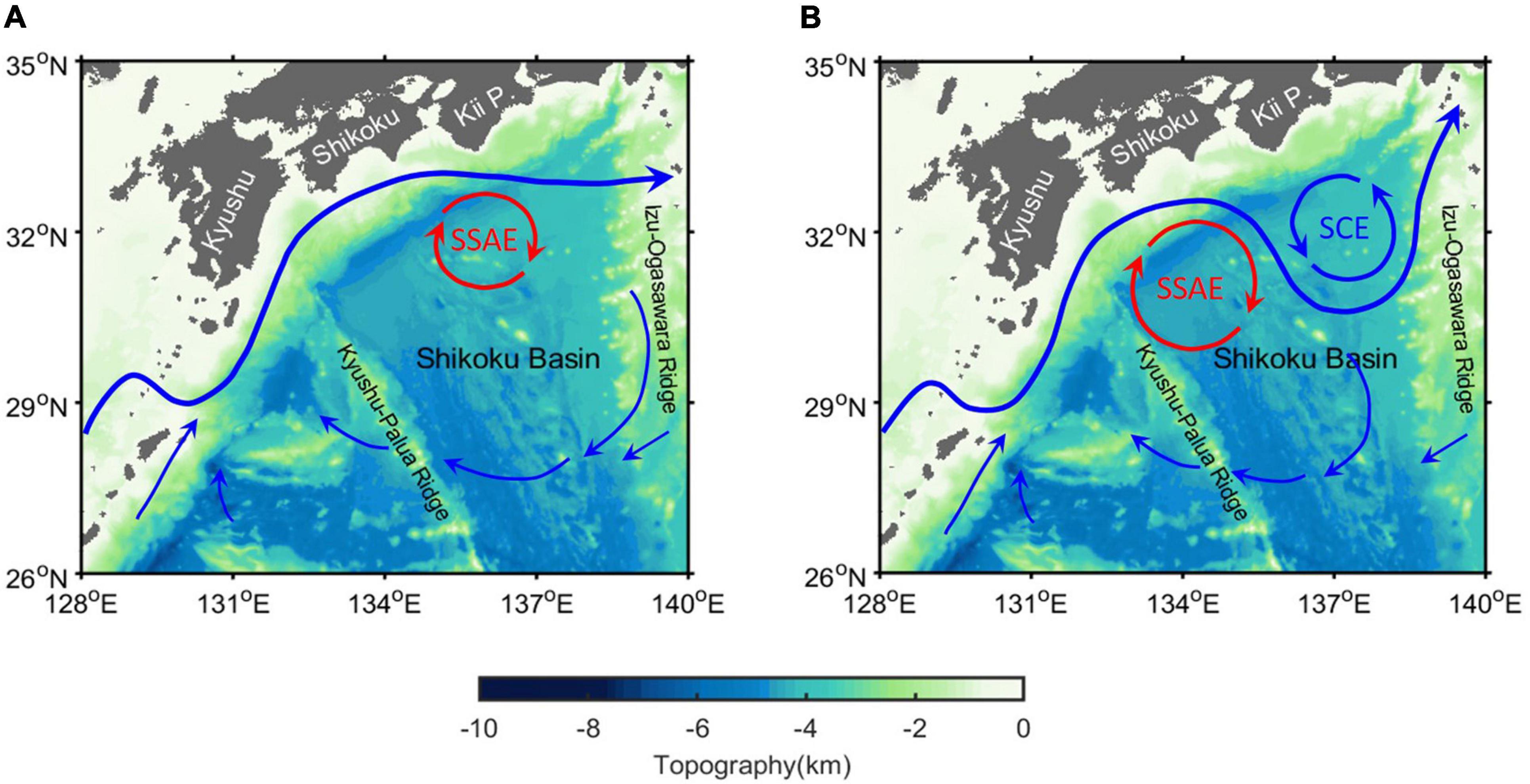
Figure 1. Schematic diagrams of the sea surface currents (blue curves) and topography (color) for the (A) NLM and (B) LM paths in the region off the southern coast of Japan. The subsurface anticyclonic eddy (SSAE) and enhanced surface (SCE) cyclonic eddy associated with the formation of the LM path are indicated by red and blue curves, respectively.
During the past few decades, scientists have paid increasing attention to the coupling relations between physical and biological processes (Lewis, 2002). The mechanisms by which mesoscale eddies influence marine biogeochemical processes can be categorized into three primary processes, namely, horizontal advection, vertical flux, and the influence of eddies on stratification and hence on upper ocean mixing. More specifically, mesoscale eddies can influence biogeochemical processes through the following mechanisms: eddy advection of nutrients, phytoplankton, and other biological tracers by the horizontal rotational velocity of eddies (Chelton et al., 2011); eddy pumping presented as an upward or downward nutrient flux induced by isopycnal displacement as an eddy forms (McGillicuddy et al., 1998, 1999; Siegel et al., 1999); the trapping of ecosystems by nonlinear eddies, of which the rotational velocities are faster than the eddy propagation speed, from their region of formation (Early et al., 2011; Gaube et al., 2014); eddy-induced Ekman pumping, which arises from convergence or divergence induced by wind and surface current interactions (Stern, 1965; Martin and Richards, 2001; McGillicuddy et al., 2007; Mahadevan et al., 2008; Morel and Thomas, 2009); eddy strain-induced pumping resulting from a cross-front ageostrophic secondary circulation, which causes upwelling/downwelling along the light/dense side of the front, generating upward nutrient fluxes and increased chlorophyll (CHL) concentrations along the light side of the front (Zhang et al., 2019); and the influence of eddies on mixing through alterations to the mixed-layer depth that impacts nutrient fluxes and, potentially, also modulates light availability (Levy et al., 1998; Gaube et al., 2013).
Chen et al. (2007) found that the cold eddy generated in the Luzon Strait can significantly increase the primary productivity. Lin et al. (2010) studied a phytoplankton bloom produced by an anticyclonic eddy injection in the oligotrophic area of the northern South China Sea. Xiu and Chai (2011), using a coupled three-dimensional physical-biogeochemical model, concluded that the modeled depth-integrated (0–125 m) CHL, zooplankton, new production, and silicate uptake were significantly enhanced in the cyclonic eddies and reduced in the anticyclonic eddies. Kouketsu et al. (2016) reported that high (low) surface area-averaged CHL concentrations were frequently observed in the core of cyclonic (anticyclonic) eddies in the Kuroshio Extension region. Based on historical cruise observations with mesoscale eddies detected by altimeters in the North Pacific, Huang and Xu (2018) showed that the depth-integrated CHL anomalies in the euphotic layer of eddies are less than ± 10%, and the integrated responses of CHL to eddies decline from ocean boundaries to the oligotrophic open ocean in the North Pacific. Using biogeochemical (BGC-Argo) floats, Xiu and Chai (2020) showed that mesoscale eddies can significantly affect the subsurface CHL maximum and subsurface biogenic particles in the central North Pacific Subtropical Gyre.
Critically, most previous studies have focused on the effect of surface eddies on CHL, or failed to distinguish different eddies, while two types of anticyclonic eddies can be differentiated based on the vertical distribution of their hydrographic signals: regular surface eddies and subsurface-intensified eddies. Regular surface eddies are characterized by expressing the largest isopycnal deformation near the surface, either upward or downward, depending on eddy polarity. Subsurface-intensified anticyclonic eddies, however, appear as positive sea level anomalies with deepening of the main pycnocline and shallowing of the seasonal pycnocline (Sweeney et al., 2003; McGillicuddy et al., 2007; Assassi et al., 2016); similar to surface cyclonic eddies, these eddies can also result in phytoplankton blooms and enhance production via the convex of the isopycnals. For example, in the southern Bay of Biscay (Rodriguez et al., 2003), a twofold enhancement of phytoplankton biomass was detected in the subsurface CHL maximum layers at the core of an anticyclonic eddy, and this enhancement was related to the injection of nutrients into the euphotic layer due to pycnocline doming. There has been a long-standing anticyclonic eddy exists in the region south of Japan; however, due to the limited availability of temporally continuous biogeochemical parameter profile data, the three-dimensional biogeochemical structure of this eddy and its contributions to biogeochemical cycles have never been systematically investigated. A complete depiction of the biogeochemical structure of this subsurface eddy is critically required, especially if eddy-associated biogeochemical cycles are to be understood. In this study, three-dimensional biogeochemical model data were used to evaluate the impacts of this long-standing eddy. We first tracked the subsurface anticyclonic eddy and then analyzed the corresponding physical and biogeochemical responses. The remainder of this paper is organized as follows: Section “DATA AND METHODS” briefly describes the information of the data and methods used in this study. The physical and biogeochemical properties of the anticyclonic eddy are in presented in Section “Physical Properties” and Section “Biogeochemical Properties,” respectively. Section “Chlorophyll Aggregation Below the ZEU in Winter” includes the mechanisms by which the anticyclonic eddy-induced CHL aggregates below the euphotic layer in winter. Summary and discussion are provided in Section “SUMMARY AND DISCUSSION.”
Data and Methods
BGC-Argo
Measurements from two BGC-Argo floats (ID: 2902750 and 2902754) were obtained from the Coriolis Global Data Assembly Centre (GDAC) FTP server1 to validate the accuracy of the biogeochemistry model data. In addition to temperature and salinity, these two floats simultaneously measured CHL concentrations (units: mg m–3) and particulate backscattering coefficient at 700 nm [bbp (700); units: m–1]. Nitrate (NO3; μmol kg–1) and dissolved oxygen (DO; units: μmol kg–1) were also measured by float 2902754. The average sampling rates of the two floats were approximately 2 days and ranged from 1-5 days. The two floats sampled from the surface to ∼1,000 m. The observed trajectories of these two BGC-Argo floats and the simultaneous satellite sea level anomaly (SLA) associated with eddy are shown in Figure 2. The BGC-Argo2902750, which was deployed in the region south of Japan on September 9, 2018, was quickly entrained into the 200−300-km anticyclonic eddy, and we studied and stayed in the eddy until the end of April in 2019; this float was successfully recovered in early June (Figures 2A,C). BGC-Argo 2902754 was released to the Northwest Pacific on August 30, 2018 and traveled for more than 2 years until March 12, 2021. From April to November of 2019, the float was rapidly captured by a cyclonic eddy intensified with the formation of the LM path (Figures 2B,D).
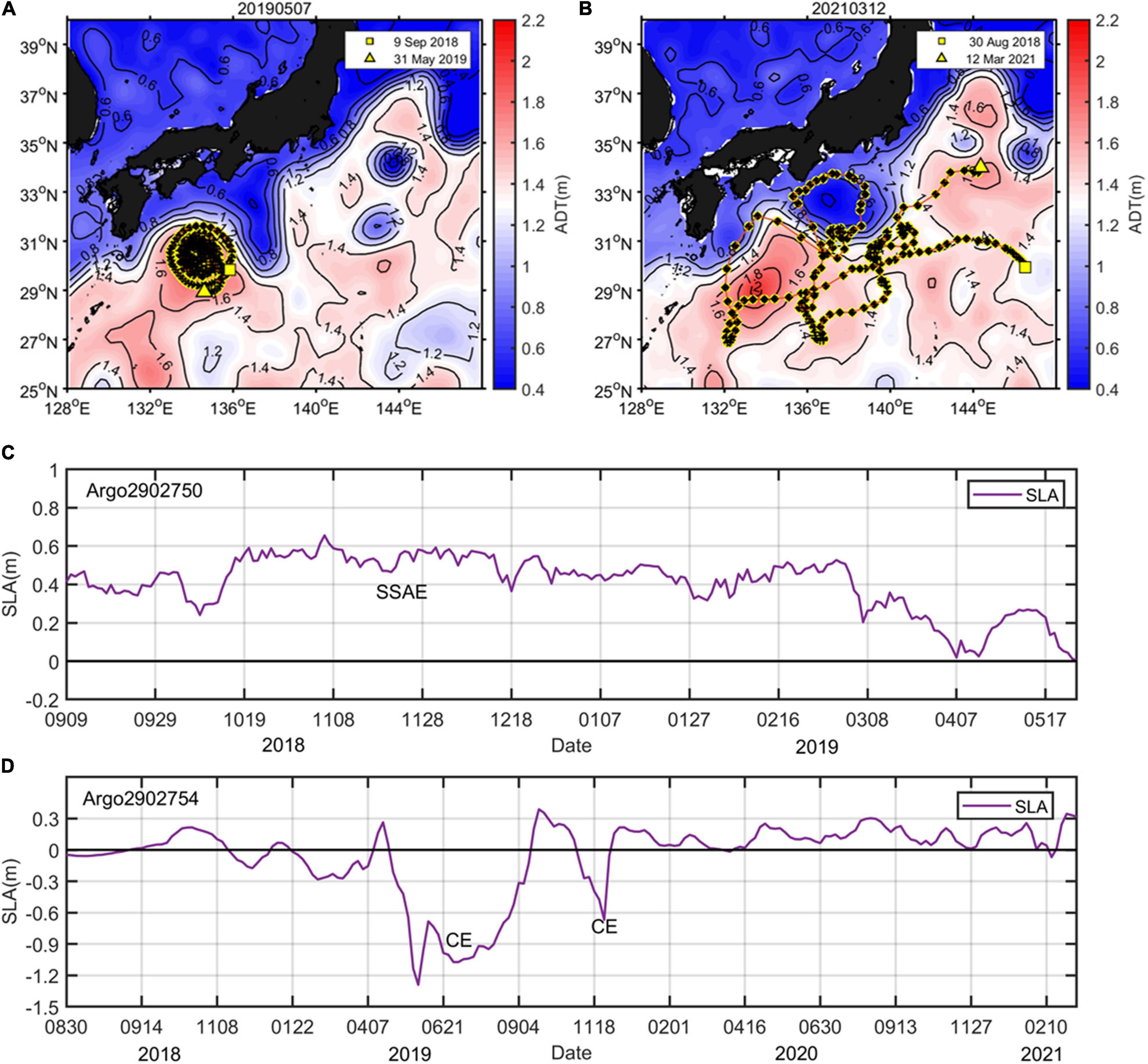
Figure 2. Tracks and the simultaneous time series of SLA of the BGC-Argo 2902750 (A,C) and BGC-Argo 2902754 (B,D) deployed in the Northwest Pacific. The background represents the absolute dynamic topography (ADT; contour and color, units: m) on the specific day of observation. The location of the first and last profiling of the floats is marked by squares and triangles, respectively.
Common and specific quality control tests have been performed on the BGC-Argo-measured variables, and we used only data with “good quality” flags. Additionally, the floats profiled at night (around 22:00–0:00 local time) to avoid phytoplankton fluorescence non-photochemical quenching and CHL profiles were dark corrected based on the on-float measurement before deployment, and further corrected based on match-up satellite CHL data using nonlinear regression function (Xing et al., 2020).
Model Data
Hydrological Data
The three-dimensional daily mean fields of temperature: salinity, zonal, and meridional velocities, as well as two-dimensional daily mean fields of mixed layer depth, were obtained from the Copernicus Marine Environment Monitoring Service (CMEMS) global physical analysis and coupled forecasting product. The coupled modeling system being used to provide the analysis and forecast products is the Met Office Coupled Atmosphere-Land-Ocean-Ice data assimilation system (CPLDA). The scientific and technical implementation of the V3.1 system is described in Lea et al. (2015). These data have a horizontal resolution of 1/4 degree and 43 vertical levels and covered the period from December 2015 to December 2020. The model includes multivariate data assimilation, which consists of a SEEK filter analysis of along-track SLA and sea surface temperature (SST), together with in situ temperature and salinity observation profiles. The altimeter reference period for the assimilated SLA is 20 years (Rio et al., 2014). The assimilated SST is taken from the CMEMS Thematic Assembly Centre (TAC) daily level-4 Operational Sea Surface Temperature and Ice Analysis (OSTIA) composite product (Donlon et al., 2012). The model bathymetry is DRAKKAR v3.3, which is based on the ETOPO1 dataset with additional data in coastal regions from the General Bathymetric Chart of the Oceans (GEBCO).
Compared with observation from a subsurface, mooring system was deployed at 25°N, 146°E from April 2017 to June 2018 (Supplementary Figure 1); the product agrees well with it in terms of temporal variation in temperature [correlation coefficient: 0.76; root mean square difference (RMSD): 0.46°C] and salinity (correlation coefficient: 0.66; RMSD: 0.04 psu). Meanwhile, this product could reproduce the important features of the Kuroshio system, including its spatial pattern of sea surface velocity in NLM and LM path south of Japan (Supplementary Figure 2).
Biogeochemistry Data
The CHL (units: mg m––3) concentration data were downloaded by file transfer protocol (FTP) from the CMEMS2 global ocean biogeochemistry analysis and forecast product (001-028), which was produced at Mercator-Ocean (Toulouse, France). This product is displayed on a regular grid at 1/4 degree resolution, with 50 vertical levels ranging from 0 to 5,500 m, on the global ocean, and includes daily and monthly mean fields of the 10 following biogeochemical variables over the period from January 2017 to the present: CHL, nitrate, phosphate, silicate, dissolved oxygen, dissolved iron, primary production, phytoplankton, PH, and surface partial pressure of carbon dioxide. This product is based on the pelagic interactions scheme for the carbon and ecosystem studies (PISCES) biogeochemical model [available on the Nucleus for European Modeling of the Ocean (NEMO) modeling platform3 ] and was forced offline at a daily frequency by CMEMS global physical analysis product coarsened at 1/4 degree, with singular evolutive extended Kalman/incremental analysis updating (SEEK/IAU) data assimilation of global ocean CHL data obtained from satellite observations. In addition, the time series is aggregated in time in order to reach a two full years’ time series sliding window. In this study, the CHL fields were log10 transformed, which accounts for the highly skewed distributions of the untransformed data that can occur in many regions of the global ocean, especially in near-coastal regions (Campbell, 1995). The detailed validation of the model data was conducted in Section “Biogeochemical Properties.”
ZEU Data
The ZEU is the depth of the euphotic layer (m), i.e., this subsurface parameter used in this study was obtained from the Glob-Color dataset4. The ZEU was computed from the corresponding merged CHL-OC5 products (Morel et al., 2007) using the following empirical equation with y = log10 (CHL-OC5):
Ancillary Datasets
The following ancillary data were used in this paper; the SLA and absolute dynamic topography (ADT) data used in this study were provided by the Archiving, Validation, and Interpretation of Satellite Oceanographic data (AVISO) from January 2017 to December 2019 with spatial and temporal resolutions of 0.25° × 0.25° and 1 day, respectively; temperature and salinity data provided by the World Ocean Atlas 2018 (WOA18, 1° × 1°,5) were used to estimate the background profile; data on the daily mainstream location of the Kuroshio were provided by the Hydrographic and Oceanographic Department of Japan6; and 12 h, 0.25° × 0.25° air-sea net heat flux (Qnet) and 10-m wind speed were provided by the ERA5 and were sourced from the European Centre for Medium-Range Weather Forecasts (ECMWF).
Eddy-Tracking and Construction Method
The eddy identification followed in this study mainly refers to the method proposed by Nencioli et al. (2010). This method is based on eddy vector geometry and has great advantages over the commonly used Okubo-Weiss method in terms of its correctness and accuracy (Souza et al., 2011). First, four constraints on the geometry of velocity vectors are defined to determine an eddy center, which was defined as the minimum velocity in a given region that extends up to a certain grid point. For more details, readers can refer to Nencioli et al. (2010). Once the center is identified, we then search for the outermost closed streamline around the center, and a tracking algorithm is conducted. If the velocity magnitudes cease to increase in the radial direction, this location can be regarded as the eddy boundary. We applied this method to obtain eddy parameters, including the location, amplitude, radius, intensity, and boundary locations of the eddy.
In order to obtain the three-dimensional physical and biogeochemical structure of the eddy, we searched the profiles located in the range of twofold radius and calculated the relative zonal and meridional distance, ΔXE and ΔYE, respectively, of profiles to the eddy center (defined at ΔXE = YE = 0). All of the profiles were then used for composition. To eliminate the influence of radius on the composite result, ΔXE and ΔYE are divided by the corresponding radius R so that they are dimensionless. After that, for profile surfacing at the boundary of eddy, it shall meet the condition . To obtain the eddy-induced three-dimensional structures in different months, all profiles in the respective months on the eddy-coordinate space (ΔXE, ΔYE) were mapped onto 0.1 × 0.1 grid using the objective analysis (Barth et al., 2014). Also, at each depth, anomaly data were treated as outliers and removed if they were more than three times away from either the first or the third quartile. Thus, for each month, a unique three-dimensional composite structure was obtained.
Results
Physical Properties
There was a long-standing anticyclonic eddy in the Shikoku Basin, although its strength and location will be significantly influenced by the Kuroshio paths south of Japan; this eddy is closely related to the SRG, which is associated with the particular ocean bottom topography south of Japan.
From January 2016 to December 2019, this long-standing anticyclonic eddy was detected from ADT and velocity images, with an average radius of approximately120 km and amplitude of 20 cm (defined as SLA difference between the eddy center and periphery), locating around 30°−32°N, 134°−136°E off Shikoku (Supplementary Figure 3). The variations in the radius, amplitude, strength, latitude, and longitude of the center of this anticyclonic eddy over its lifetime are shown in Figure 3. If the southernmost position of the Kuroshio axis is located south (north) of 32°N, it is classified as a meander (non-meander) path (Sugimoto and Hanawa, 2014). With the development of the LM path (gray background in Figure 3C), the radius, amplitude, and intensity (the ratio of the amplitude to the radius) of the anticyclonic eddy increase gradually as the position shifts southwest. While, according to the idea of the self-sustained oscillation mechanism (Qiu and Miao, 2000), the strength of the SRG increases continuously when the Kuroshio is in its straight path state, corresponding to the decreasing trend of the spatially averaged relative vorticity. During the transition period from the NLM to the LM path, a sudden release of velocity shear corresponds well to the weakening of the SRG, which plays a key role in modulating the Kuroshio path variations. We tried to explain that the trends observed in the anticyclonic eddy intensity are opposite to those of the SRG from the perspective of energy conversion.
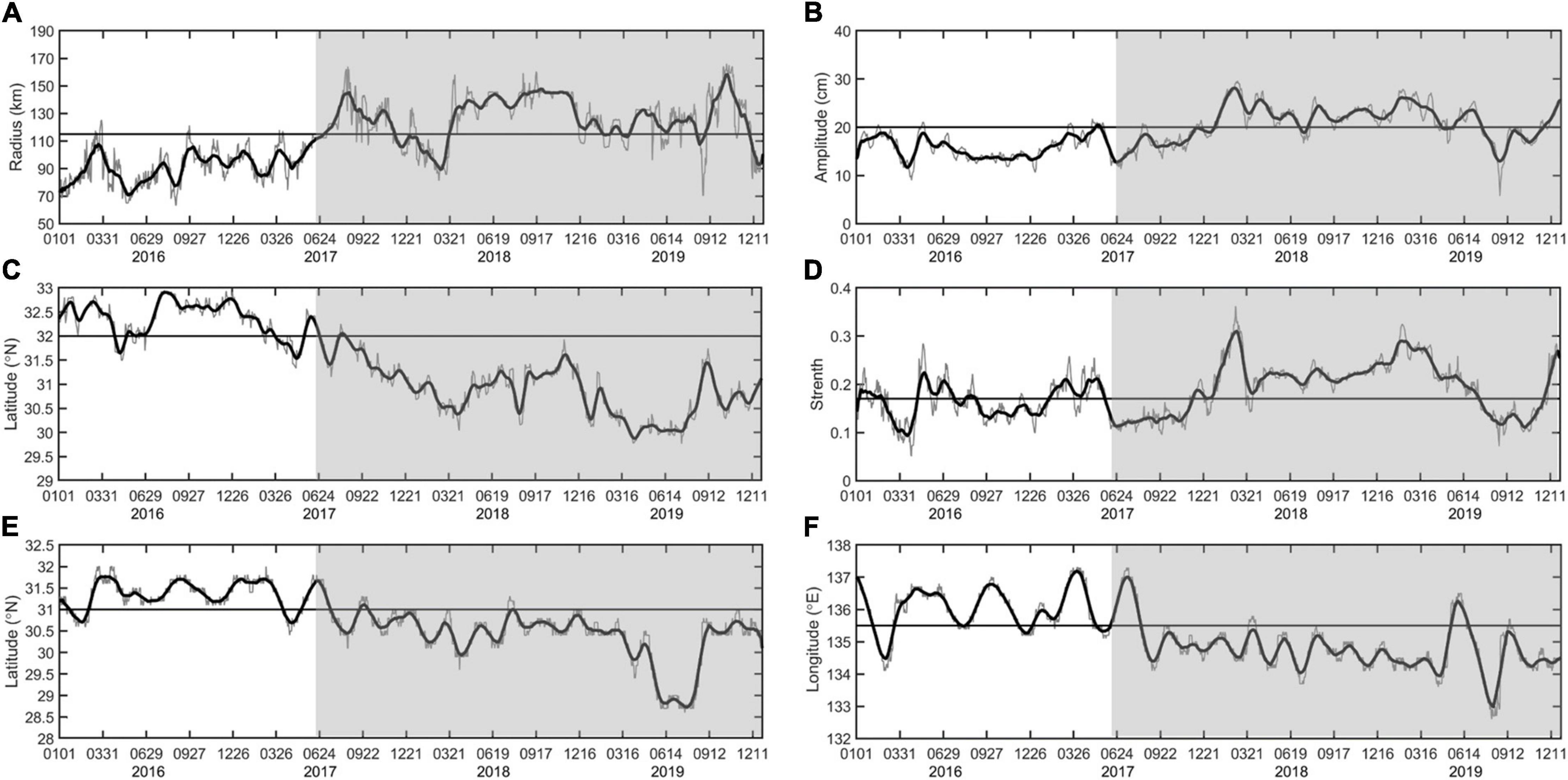
Figure 3. Variations in the (A) radius, (B) amplitude, (C) southernmost location of the main axis of the Kuroshio between 135° and 142°E, (D) strength, (E) center latitude, and (F) center longitude during the lifetime of the studied anticyclonic eddy. The LM path periods are shaded in gray.
Previous studies have indicated that baroclinic instability is a necessary component on the formation of the LM path (Yoon and Yasuda, 1987; Tsujino et al., 2006). Eddy energetics analysis is a useful tool for evaluating flow instabilities (Lorenz, 1955, 1960). However, it is difficult to define the background field due to the great variability that exists in the path of the main Kuroshio axis south of Japan. Tsujino et al. (2006) suggested decomposing an instantaneous field into the field at the previous time step as a mean field and the deviation from this previous field as an eddy component. Here, we adopted the same method for the monthly mean velocity and analyzed the local energetics at each time step. The barotropic (BT) conversion rate from the mean kinetic energy (MKE) to eddy kinetic energy (EKE), which indicates the barotropic instability, is defined as follows:
where ρ0 denotes the density, () is the mean zonal (meridional) velocity, and u′(v′) is the perturbed velocity in the eddy field. The baroclinic (BC) conversion rate from mean potential energy (MPE) to eddy potential energy (EPE), which is associated with the baroclinic instability, is calculated as follows:
where g is the gravity acceleration, N2 is the Brunt-Vaisala frequency squared, and ρ with the overbar and prime denote the mean and eddy components, respectively. More details of the above eddy energy conversion rate equations and the specific calculation process can refer to Tsujino et al. (2006).
The spatial distributions of the two energy conversion rates described above were calculated by Equations (2) and (3), and the energy conversion distribution areas were located near the main axis of the Kuroshio, which may have been due to the relatively large velocity in this region (Li et al., 2014). In addition, the volume-integrated (upper 1,000 m) energy conversion rates were calculated over the area (30°–35°N, 132°–140°E) (Figure 4). We found that the energy conversion rate of BC over the volume integral was larger than that of BT, indicating that the BC instability plays a major role in the formation of the LM path. Sharp increases in these two conversion rates can be seen before the onset of the LM path, demonstrating the transfer of energy from the mean field to the eddy field. It is possible that the enhanced strength of the anticyclonic eddy resulting from the eddy kinetic energy was provided by the dramatic increase observed in the positive BC conversion rate.
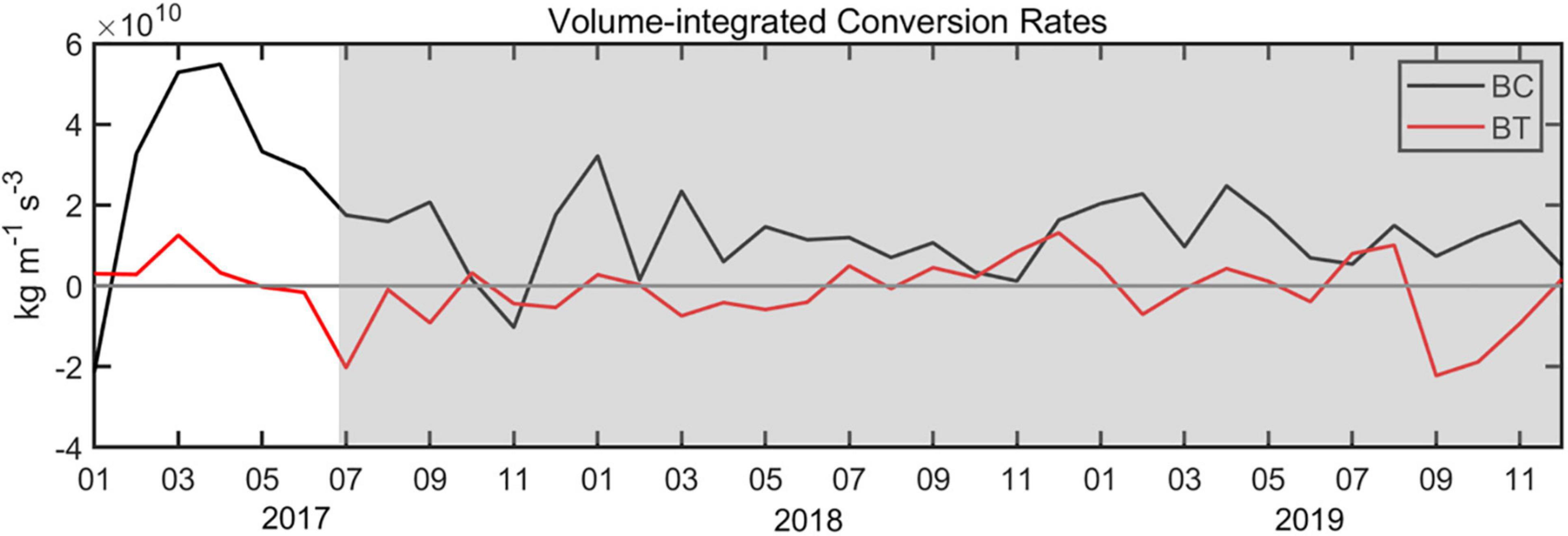
Figure 4. Time series of two conversion rates volume-integrated (upper 1,000 m) over the area (30°–35°N, 132°–140°E). LM path periods are shaded.
After having analyzed the variations in the anticyclonic eddy intensity when Kuroshio takes different paths, we subsequently tried to investigate differences in temperature and salinity structure of it. The composited monthly temperature and salinity anomalies vertical section structures of the studied anticyclonic eddy in winter (February), spring (May), summer (August), and autumn (November) during the LM path period (2018–2019) are displayed in Figure 5, respectively. As the figure shows, this is a typical subsurface anticyclonic eddy (SSAE), characterized by maximum temperature and salinity anomalies core as well as maximum velocity (Supplementary Figure 4) in the subsurface. And the SSAE is fairly strong, with magnitude of maximum temperature and salinity anomalies exceeding 4°C and 0.3, respectively. The comparison results showed that the positive temperature and salinity anomalies above 800 m caused by the SSAE during the NLM path years (2016–2017, Figure 6) had smaller magnitudes and wider horizontal scales of the core; robust negative temperature and salinity anomalies resulting from the influence of the Kuroshio are clearly seen on the right side of the figure in the LM path period (Figure 5, February, May, and August). Notably, significant seasonal variation exists in the central potential density structure in the LM path period; the SSAE shows a normal concave isopycnal structure from January to April and a convex lens structure from May to December but is less pronounced in NLM path periods.
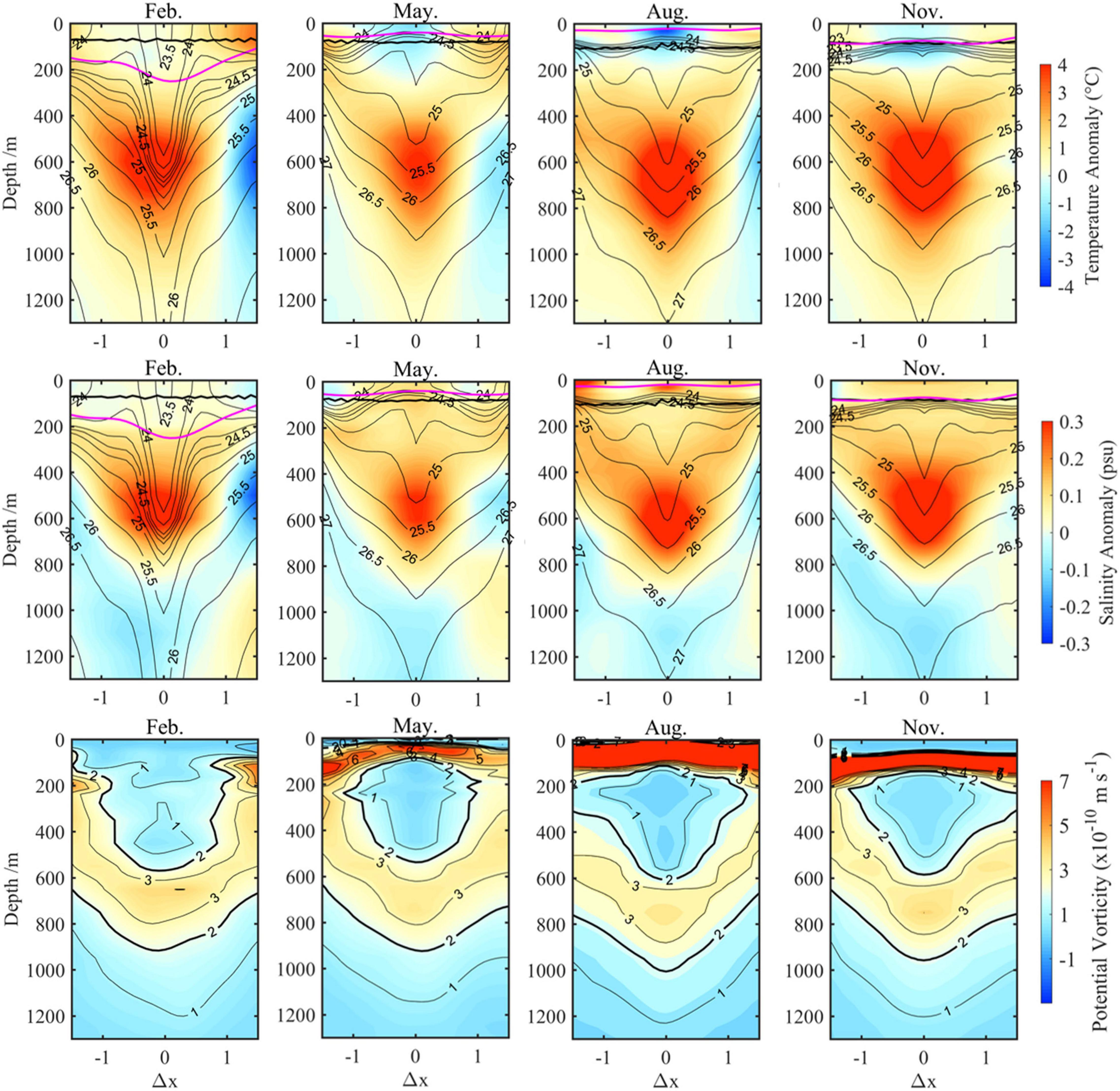
Figure 5. Composite monthly vertical sections of SSAE in February, May, August, and November during the LM path period. Top-to-middle rows show zonal sections of temperature anomalies (color, unit: °C), salinity anomalies (color, unit: psu), and potential density (contour, unit: kg m–1). The magenta lines indicate the MLD, and the black lines indicate the base of ZEU; the bottom row shows the potential vorticity (color and contour, unit: m s–1).
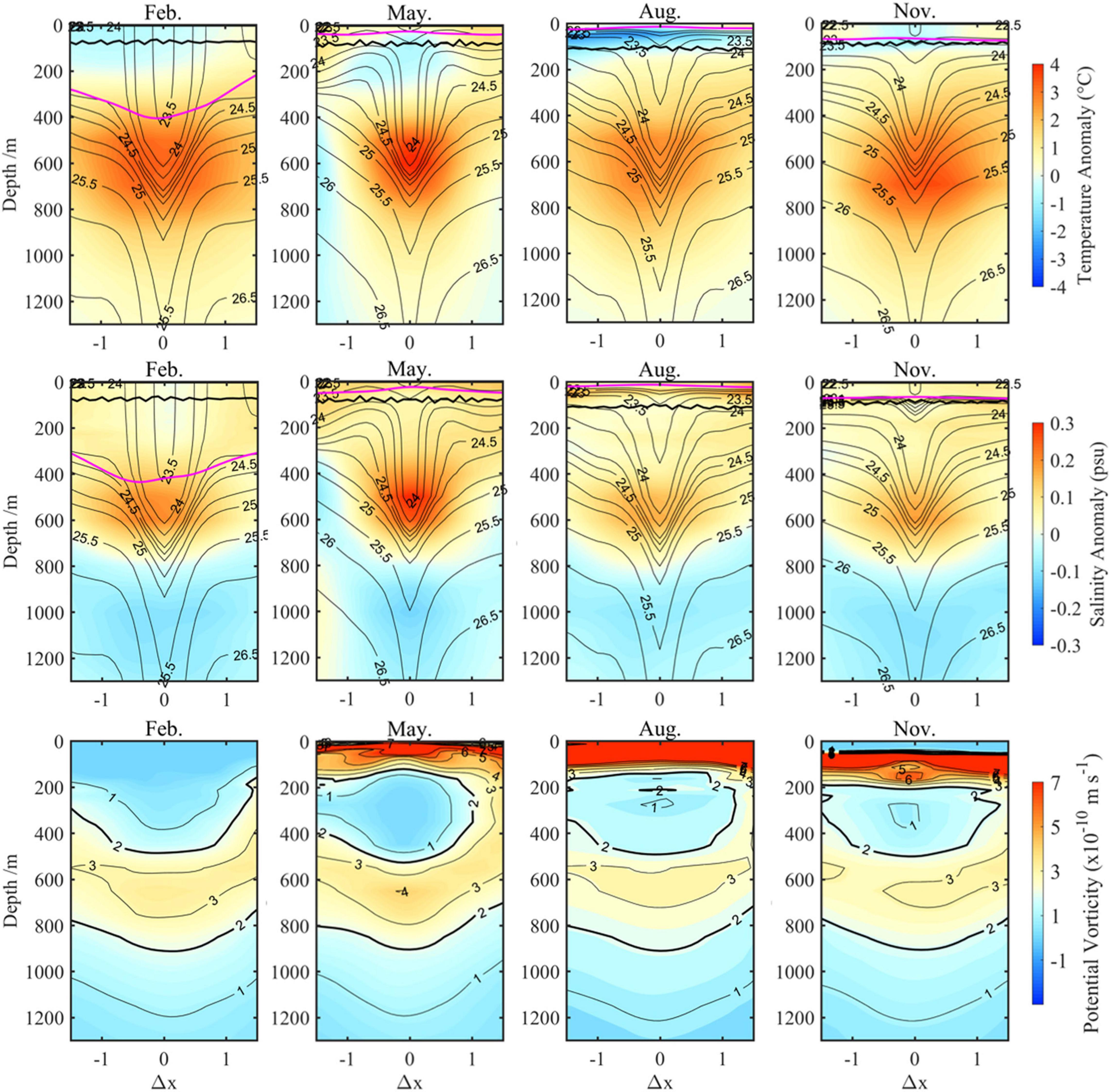
Figure 6. Same as Figure 5 but during the NLM path period.
The lens structure of isopycnals is typical for subsurface eddies, and the existence of the low-potential vorticity (PV) inside the eddy center was thought to be the major reason for this structure. Relative vorticity is usually much smaller than planetary vorticity in most of the interior of the ocean, if ignoring the effects of the relative vorticity; the PV has the following expression (Pedlosky, 1996; Stewart, 2008; Nan et al., 2017):
where ρ denotes the potential density. The relative vorticity (defined as ζ) of the SSAE is negative (clockwise horizontal velocity, Supplementary Figure 4); thus, it always has the opposite sign to the planetary vorticity, which means the PV anomaly caused by relative vorticity always has the same sign with the PV anomaly caused by the lens-shaped density field at the eddy center (Zhang et al., 2017). Therefore, failing to consider the influence of the relative vorticity causes only the amplitude of the absolute PV anomaly to be underestimated, indicating that only some weak subsurface eddies may be missed; at the same time, the stronger SSAE detected by Equation (4) is reliable. From the composite vertical PV sections shown in the bottom row of Figure 5, the seasonal variation in the central potential density structure of SSAE may have been related to the subduction of low-PV North Pacific Subtropical Mode Water (STMW).
Generally, anticyclones deepen the mixed layer depth (MLD), whereas cyclones thin it, with the magnitude of these eddy-induced MLD anomalies being largest in winter (Gaube et al., 2019). Furthermore, the extent to which eddies modulate the MLD is linearly related to the sea surface height amplitude. Eddy-centric composite averages from Figures 5, 6 also reveal that the largest MLD anomalies occurred at the eddy center and decreased with increasing distance from the center. As a result, due to the unique seasonal variations in the central potential density of SSAE, this fairly strong eddy could deepen the mixed layer by an average of more than 100 m from January to April; in other seasons, however, it has the contrary effects.
Biogeochemical Properties
A comparison with existing observations was conducted to demonstrate the accuracy of the model data before using it to study the biogeochemical structure of SSAE. The model could reasonably reproduce the general spatial pattern of CHL, including the relatively high CHL concentrations in the coastal region, the low values in the deep basin, and the westward pointing “arrowhead” shape of the CHL tongue in the tropical band of the Pacific Ocean (Supplementary Figures 5, 6). The modeled vertical distributions trend of CHL, NO3, and DO agrees well with the compared BGC-Argo, but was overall underestimated or overestimated when compared to BGC-Argo (Figure 7). The temporal variabilities, especially on the seasonal cycle at mid-latitudes and high-latitudes, of model CHL and two BGC-Argos were similar (r = 0.5, p < 0.01; correlation coefficient even reaching.68 above 100 m): spring or winter bloom. The model also showed fairly well temporal correlation with BGC-Argo DO (r = 0.86, p < 0.01) and NO3 (r = 0.85, p < 0.01). As the Argo observations are discrete in both temporal and spatial, the results of the vertical profiles comparison for this long time-series are valuable, although they have some discrepancies. And, from April to November of 2019, the Argo2902754 was captured by a cyclonic eddy (Figure 2D) with significantly elevated isopycnals (Figures 7E,F), and the model also responded well to this mesoscale eddy. Therefore, it is plausible to investigate the ecological effects of mesoscale eddies using model data.
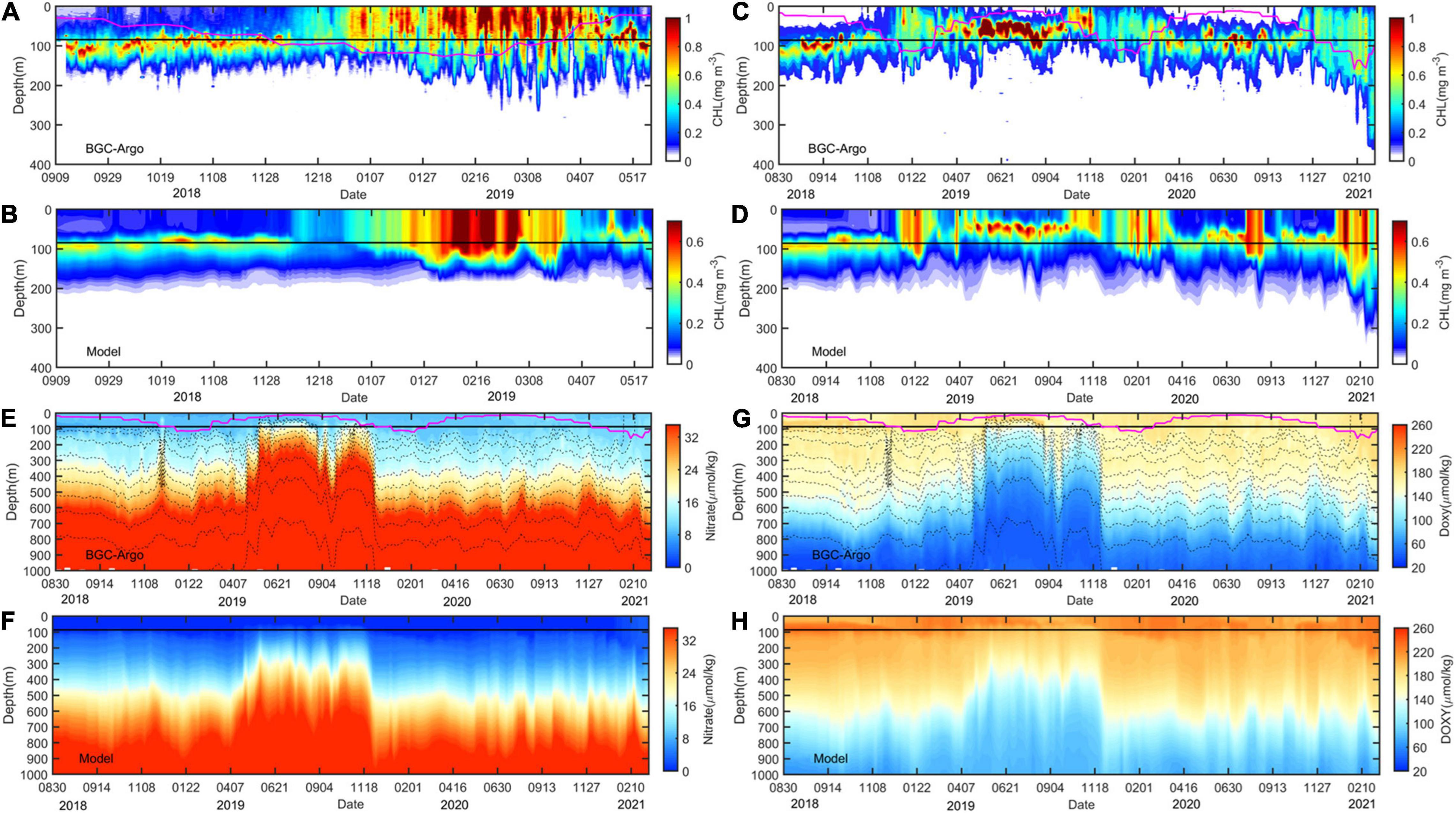
Figure 7. Comparison of time series of the modeled parameter (A–D) CHL (mg m–3), (E,F) NO3 (μmol kg–1) and (G,H) DO (μmol kg–1) with data recorded by BGC-Argo floats in the region south of Japan from 2018 to 2021. The black dashed lines in (E,G) are potential density contours. The magenta lines indicate the MLD, and the black lines indicate the base of ZEU.
In addition to the above qualitative comparison of the biogeochemistry parameters, we should also quantify the bias between the model and the observed data. To achieve meaningful quantitative results of variables, we combined measurements of other 9 BGC-Argo floats in the region of Kuroshio Extension (120°−180°E and 25°−45°N, Supplementary Table 1). Figure 8 shows the comparison between the model and profiles of BGC-Argo CHL, NO3, and DO concentrations. To estimate errors more accurately, the BGC-Argo CHL profiles were firstly corrected based on match-up satellite CHL data using nonlinear regression function (Xing et al., 2020; Xiu and Chai, 2020; Figures 8A,B), and temporally averaged CHL profiles were further compared with the model (Figures 8C,D). Overall, the model and float CHL vertical concentrations distributions compare reasonably well with a correlation coefficient of 0.71, a negative bias of 0.02 mg m–3 and an RMSE of 0.06 mg m–3, which means the model tends to underestimate the CHL concentrations; for NO3 concentrations, the model is in good agreement with a correlation coefficient of.89, a negative bias of 1.89 μmol kg–1, and an RMSE of 4.99 μmol kg–1 (Figure 8E). The model tends to overestimate NO3 for NO3 < ∼20 μmol kg–1 and to underestimate high NO3 concentrations; and for DO concentrations, the model and float are in favorable agreement with a correlation coefficient of 0.92, a positive bias of 15.56 μmol kg–1, and an RMSE of 18.74 μmol kg–1 (Figure 8F). The model tends to underestimate DO concentrations at lower levels.
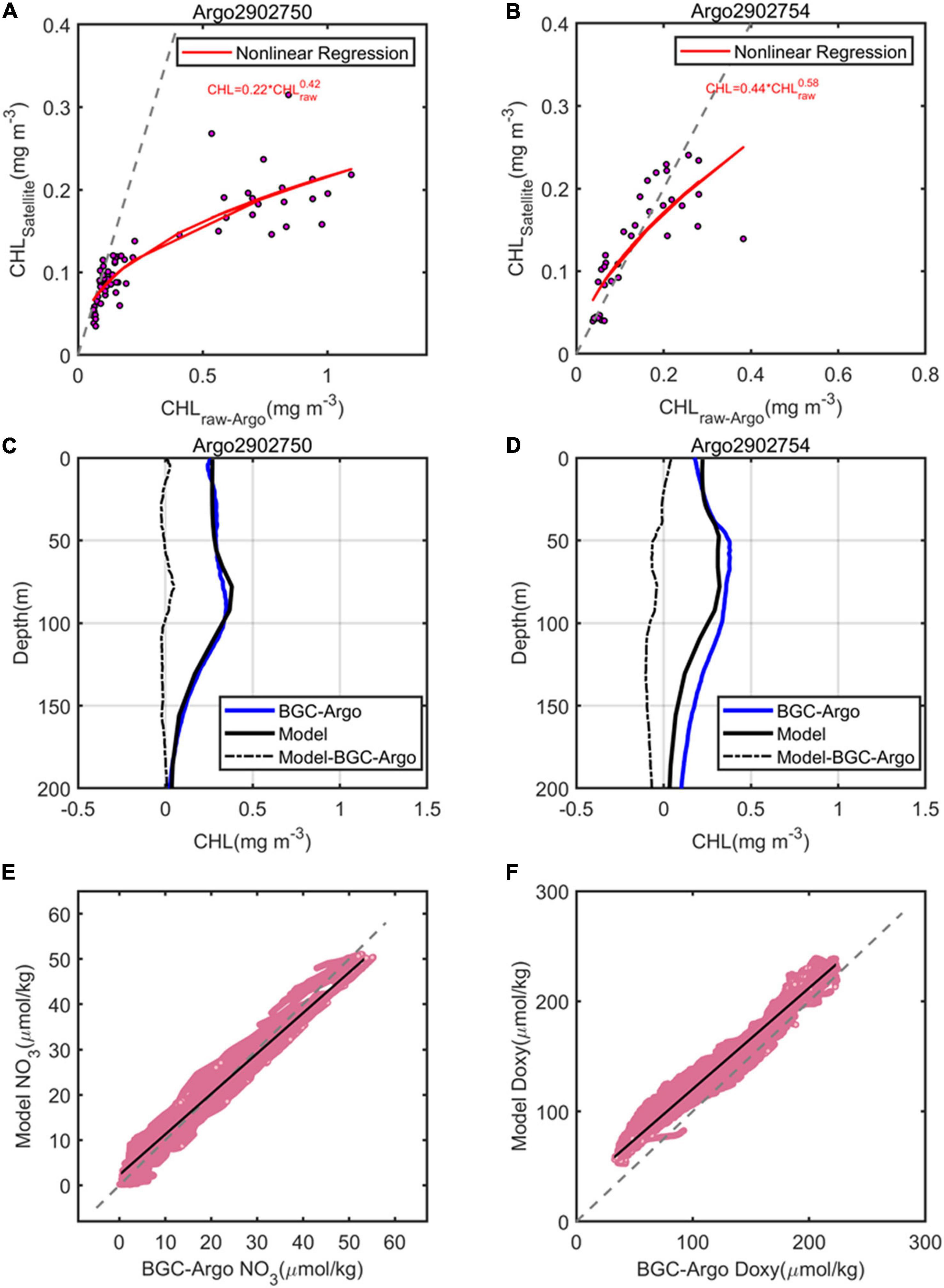
Figure 8. Comparison of (A,B) sea surface satellite CHL and (C,D) temporally averaged vertical profiles of corrected CHL with BGC-Argo 2902750 and 2902754. The red lines represent the nonlinear regression fit, and the dashed gray line represents the 1:1 line in (A,B). Model versus observed (E) NO3 and (F) DO concentrations, which show all comparisons from the surface to maximum depth of the BGC-Argo floats listed in Table S1. The black line is the least square regression fit within the data (E,F).
In the region south of Japan, there was a significant seasonal change in CHL, which increases every winter and early spring and decreased in summer (Supplementary Figure 6). Usually, persistent thermal stratification of the upper ocean means that the surface-mixed layer rarely reaches the depth of the nutricline. Therefore, the vertical distribution of CHL is not typically homogeneous and displays a pronounced maximum close to the base of the euphotic zone, which is called the subsurface chlorophyll maximum (SCM) (Figures 7A–D; Anderson, 1969; Furuya, 1990; Dore et al., 2008; Mignot et al., 2011; Xiu and Chai, 2020). Usually, in the open ocean, the depth of SCM varies over a range of 80−130 m, becoming shallower with increasing latitude; while, in near-shore regions, it ranges between 5 and 50 m (Gong et al., 2012). It should be stressed that CHL concentrations are greater in region south of the Kuroshio main axis than near-shore regions at depths below 50 m (Supplementary Figure 6). The SCM exists throughout the year in tropical and subtropical regions. The seasonal variation of the SCM depth is significant; it is shallow in winter and deep in summer, which is proportional to the light intensity (Radenac and Rodier, 1996; Hense and Beckmann, 2008). Other than that, the depth of the SCM is negatively correlated with the depth of the mixed layer (Figures 7A,C; Qiu et al., 2018). Despite being influenced by many other factors, the SCM often results from photo-acclimation of the phytoplankton organisms in stratified waters, which induces an increase in the intracellular CHL in response to low-light conditions (Kiefer et al., 1976; Winn et al., 1995; Fennel and Boss, 2003; Dubinsky and Stambler, 2009).
It is demonstrated via our previous analysis that there is a significant seasonal variation in the dynamic structure of the SSAE; this seasonal variation determines the distribution of biochemical parameters. Therefore, we intended to investigate the seasonal variation of biochemical parameters corresponding to the dynamic structure of SSAE. Only the biogeochemical structures of SSAE during the LM path period (2018–2019) were composited here due to the lack of biogeochemical data before 2017. In the same way as before, the composite three-dimensional CHL, NO3, and DO anomaly structures of the SSAE from the surface to 150 m in February, May, August, and November during the LM path period (2018–2019) are shown in Figure 9. In February, DO within the SSAE showed positive anomalies due to the concave of isopycnals, while the CHL and NO3 concentrations also showed positive anomalies rather than their typically observed negative anomalies. The consistently higher CHL levels throughout the top and bottom of the ZEU in the center of the SSAE resulted from enhanced winter mixing; the deepened MLD was favorable to the entrance of nutrients into the ZEU from the bottom of the mixed layer. A convex lens isopycnal structure was observed from May to December in the SSAE, with convex isopycnals occurring above 200 m opposite to February. During this time period, the composite CHL, NO3, and DO structures within the SSAE showed positive anomalies around the depth of SCM (50−80 m), and elevated CHL and DO levels and reduced NO3 levels along the periphery of the eddy below the depth of SCM. According to Xu et al. (2019), they proposed two potential generation mechanisms for these CHL rings: horizontal advection and wind-current interaction. The role of advection is excluded at this depth; therefore, these CHL, DO, and NO3 rings of SSAE may have been related to wind-current interaction and sub-mesoscale process-associated vortex Ross by waves (Zhang and Qiu, 2020). Twofold to threefold increase of CHL was detected in the subsurface CHL maximum layers at the core of the SSAE, and this enhancement was related to the injection of nutrients into the ZEU due to winter mixing and the convex of isopycnals.
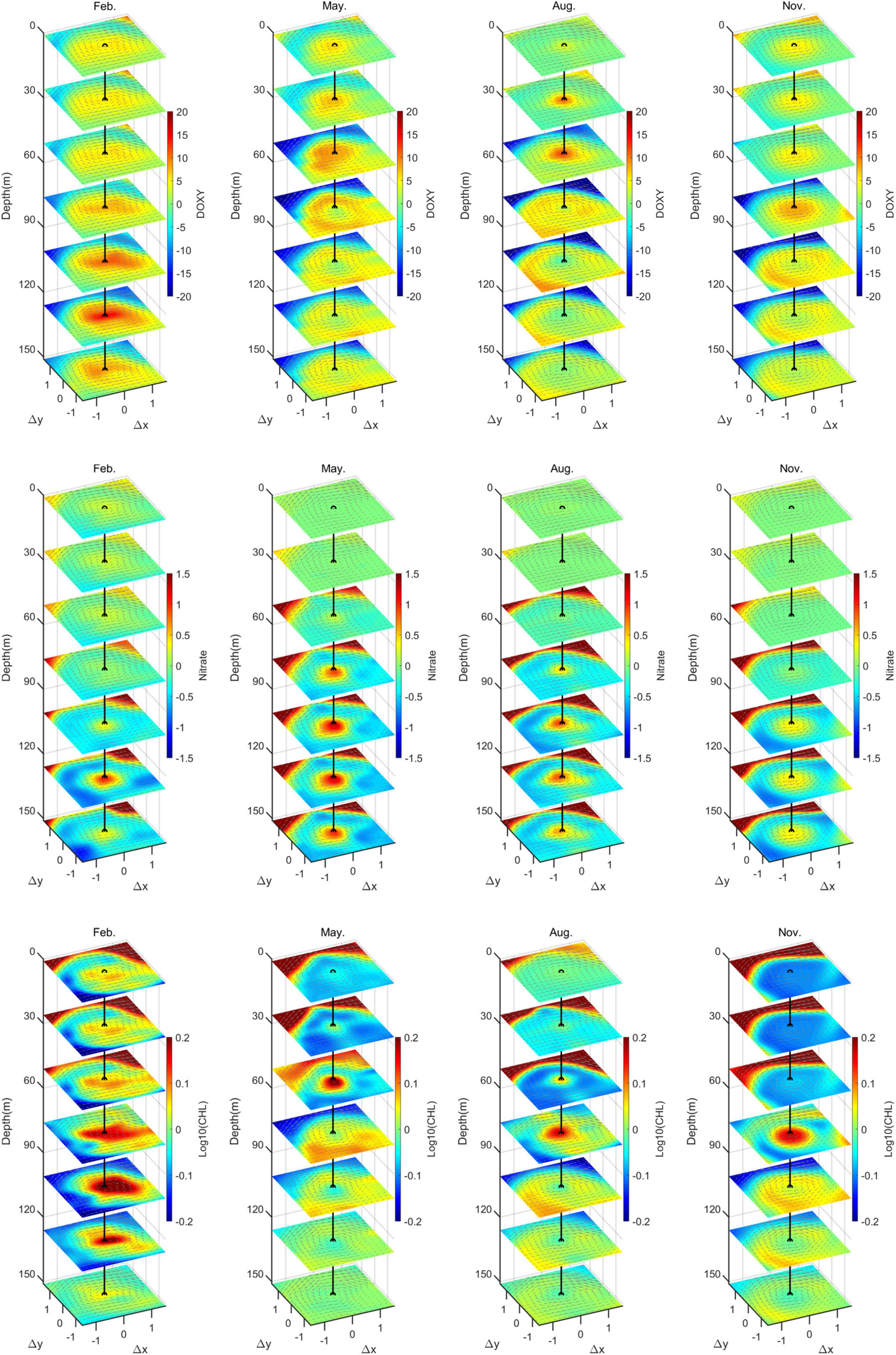
Figure 9. Composite three-dimensional anomaly structures of SSAE in February, May, August and November. From the top to the bottom, the rows show the structures of CHL (mg m–3), NO3 (μmol kg–1), and DO (μmol kg–1).
Chlorophyll Aggregation Below the ZEU in Winter
The near-surface mixed layer is the conduit by which the atmosphere influences the ocean interior, and, conversely, the ocean modulates fluxes into the atmosphere. In addition, primary production in the ocean is modulated by nutrient and phytoplankton fluxes through the base of the mixed layer and the availability of light (Dawson et al., 2018; Frenger et al., 2018; Song et al., 2018). Although there is no doubt that the mixed-layer processes are important for biological processes, the relationship between mixed-layer properties and biogeochemical parameters inside eddies remains unclear. Above, we mentioned that the depth of the SCM is negatively correlated with the MLD, and is shallow in winter and deep in summer, ranging from 50 to 200 m. Thus, it is amazing that high CHL and total phytoplankton concentrations were found at depths far below the euphotic layer (Figure 10). As we know, there is low CHL and productivity below 200 m (where CHL concentration is typically smaller than 0.1 mg m–3); thus, it is intriguing to explore this unusual event.
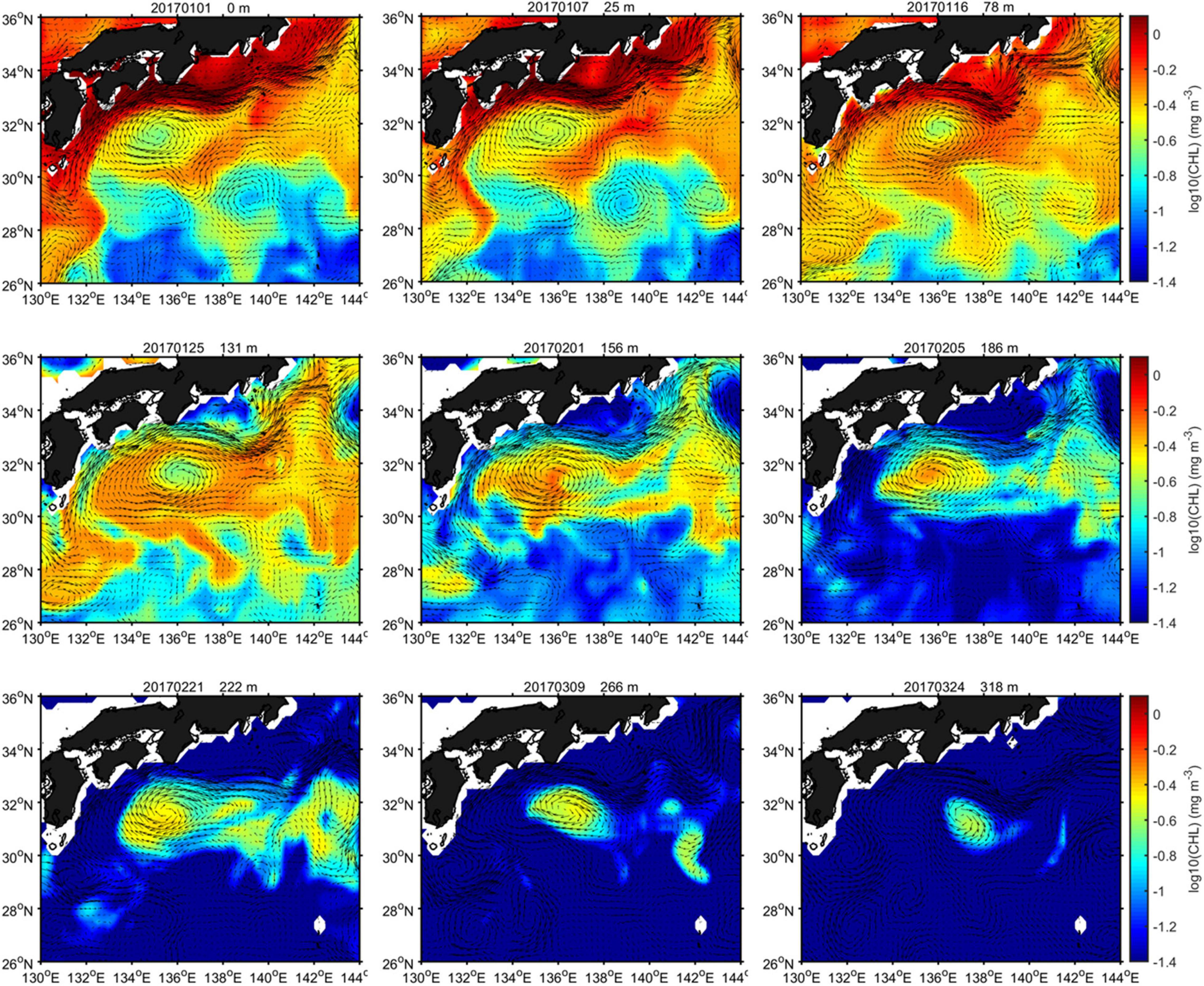
Figure 10. Spatial distribution of CHL at different depths from 1 January to 24 March 2017.
As illustrated in Figure 10, the CHL concentrations around the SSAE showed obvious downward propagation with depth from 1 January to 24 March 2017 (during the NLM period). Due to the CHL, concentrations in this area are relatively high in winter; northern coastal nutrients and plankton are entrained by the horizontal advection of the SSAE, resulting in elevated CHL along the periphery of the eddy in the initial stage; then, stirring caused a gradually uniform CHL distribution to be observed in the eddy. As the eddy intensity increased, due to the combined effect of the central downward displaced isopycnals in SSAE and winter mixing, high CHL concentrations were progressively found at depths of 222, 266, and even 318 m. Based on thickness and duration of high-CHL-level occurrences, we roughly estimated that the vertical downward speed caused by the SSAE was 2 m d–1; this speed is consistent with the magnitude of strong eddy-induced Ekman pumping (Gaube et al., 2014). Additionally, a similar phenomenon was captured from January to March 2018 (during the LM period, Supplementary Figure 7). However, the high CHL level associated with the SSAE occurred at shallower depths during this year compared to 2017. Based on our previous analysis in Section “Physical Properties,” the strength of the SSAE increases resulting from the dramatic increased positive BC conversion rate during the transition period from the NLM to the LM path. It seems to indicate that the weaker SSAE corresponds to more pronounced CHL downward displacement below the ZEU.
In order to better investigate the differences between these two processes, time series of regionally averaged CHL, total phytoplankton (concentration of phytoplankton expressed as carbon in sea water, Phyc), and MLD during January to April 2017 and 2018 are given in Figure 11. The averaged CHL, Phyc, and MLD values were derived by obtaining the daily fields located within 1.5 times the length of the SSAE radius (1.5 R). The more pronounced CHL downward displacement below the ZEU (at depths of ∼90 m) caused by the SSAE reached 320 m in 2017, resulting in the CHL levels being elevated by approximately threefold at that depth, whereas this downward propagation reached only 260 m and a nearly 2-fold-elevated CHL level in 2018. The CHL concentration was used as the best available proxy for the phytoplankton biomass; it means that this downward displacement process enables more phytoplankton at that depth. And the ultimate downward propagation depth closely fitted the MLD in the SSAE, implying that the vertical displacement of CHL may be mainly explained by the variations in the MLD (Figures 11A,B,E,F). Near-surface CHL is known to be strongly dependent on processes that control the MLD, with wind and heat fluxes having significant roles (Chiswell et al., 2015). Generally, the MLD is directly proportional to the sea surface wind stress and heat flux. To demonstrate two factors causing MLD variations, regionally averaged (over the area from 132°−140°E and 28°−35°N) 10-m wind stress and air-sea net heat flux (Qnet) were calculated in 2017 and 2018, and the results revealed that enhanced ocean heat losses and wind stresses in January and February of 2017 allowed a deeper MLD (Figures 11G–J).
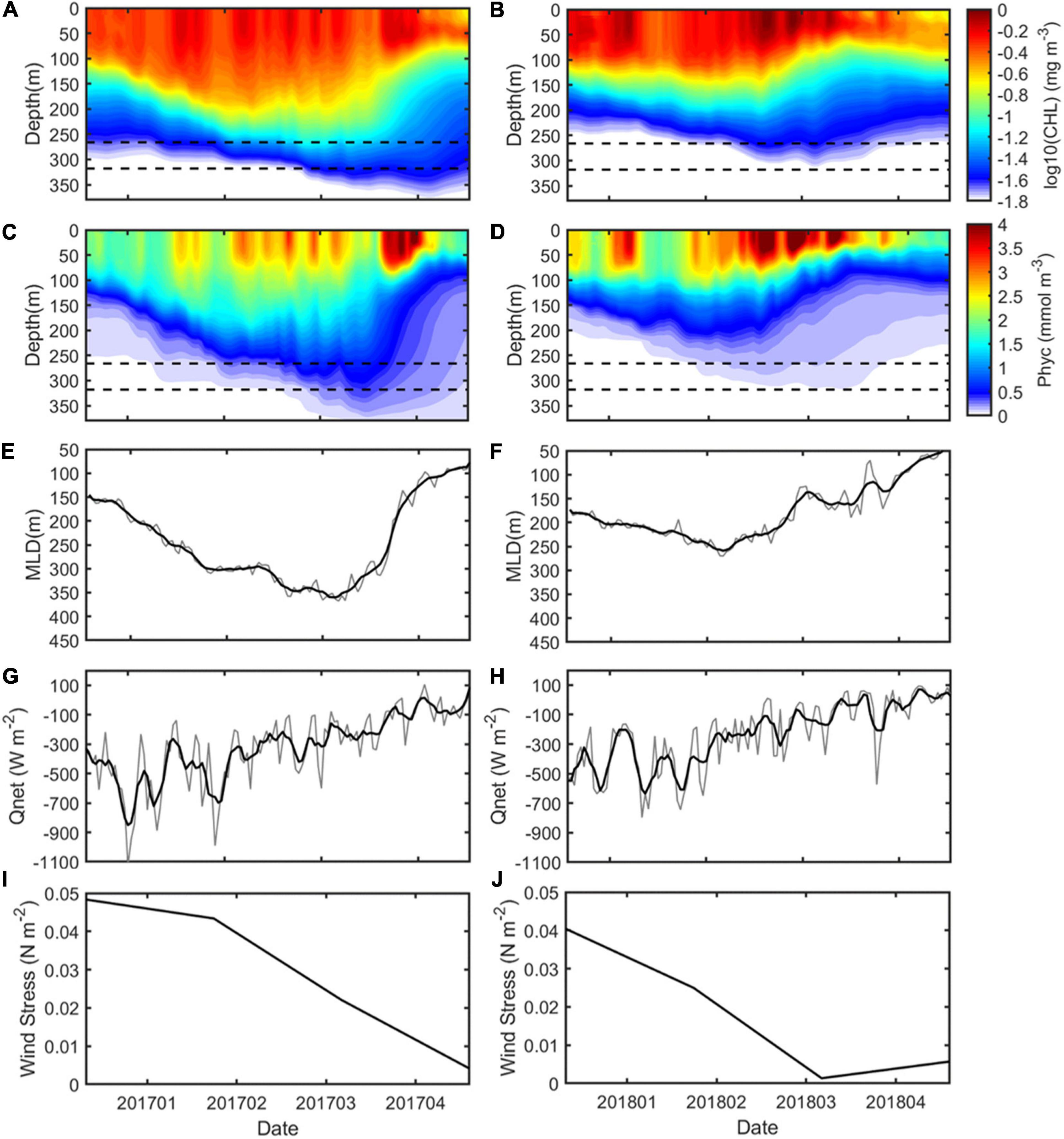
Figure 11. Time series of regionally averaged CHL, total phytoplankton (Phyc), MLD, Qnet, and wind stress in 2017 (A,C,E,G,I) and 2018 (B,D,F,H,J). The dotted lines in panels (A–D) represent depths at 266 m and 318 m.
In addition to the two factors causing MLD variations mentioned above, physically, stratification in the summer/fall months is important because it preconditions the development of the convective mixed layer during the subsequent cooling season (Qiu and Chen, 2006; Iwamaru et al., 2010). The upper ocean stratification during the preceding warm season as weaker (stronger) stratification results in a deeper (shallower) MLD in the subsequent winter; here, the July–September value is chosen to represent the condition before the onset of the cooling season. The result also suggested that the upper ocean stratification during the preceding warm season in 2017 was weaker compared to 2018 (Supplementary Figure 8), which was favorable to the development of a deeper MLD in the following winter.
Then, we have concluded that more pronounced CHL downward displacement below the ZEU associated with the SSAE mainly results from the deeper MLD in winter 2017. To further explore the relationship between the MLD and biochemical parameters inside eddies, we plot in Figure 12 the time series of NO3 and DO averaged in 1.5 times radius of the SSAE in the winter of 2017. The nutricline represents the concentration of one or several nutrients rapidly increasing or decreasing, which depends on the degree of water column stratification. When physical mixing increased in the winter of 2017, the upper mixed layer penetrated the nutricline, thereby providing a source of nutrients to the euphotic zone (Figure 12A); under these conditions, the phytoplankton became elevated throughout the upper water column. Consequently, a CHL bloom was generated in the SSAE in April 2017 (Figure 12C). Conversely, when thermal stratification increases, the upper water column is deprived of nutrients, leading to the progressive deepening of the nutricline closely paralleling the ZEU. Recent studies have suggested that CHL enrichment in anticyclonic eddies in southeastern Indian Ocean is dominated by winter mixing, which enhances the entrainment of nutrients into the euphotic zone from the bottom of the deepened mixed layer (Dufois et al., 2014, 2016). In this eddy case, both the MLDs in and out of the SSAE deepen in winter. However, the MLD in the eddy is deeper (on average, 100 m) than that out of the eddy. The deeper MLD in the eddy, closer to the deep-nutrient-rich water, may possibly lead to more nutrients being entrained into the euphotic zone and, therefore, higher CHL concentrations.
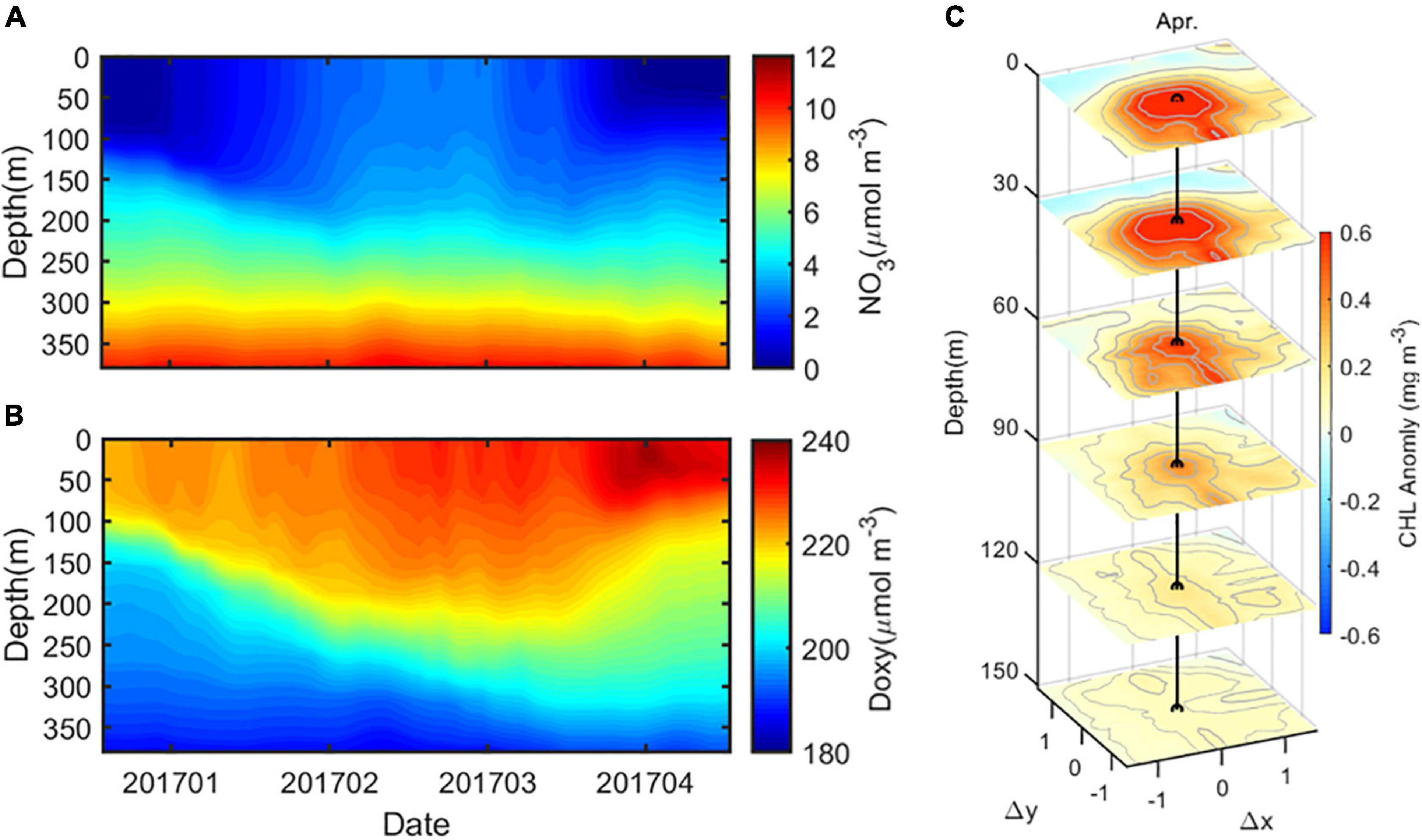
Figure 12. Time series of (A) NO3 and (B) DO averaged in 1.5 times radius of the SSAE in the winter of 2017, and (C) the composite three-dimensional CHL anomaly structure of SSAE in April 2017.
As we discussed in Section “Physical Properties,” the path of the Kuroshio south of Japan had a significant impact on the SSAE. It is worth noting that these two downward propagation processes associated with the SSAE in winter 2017 and 2018 were at different periods of the Kuroshio path; the former occurred during the NLM period on the eve of the path transition, while the latter was during the stable LM period. According to previous studies, the transition process from a straight to a meandering path is modified by stratification and bottom topography. The former enhances a small meander much more than in the barotropic case through shoaling of the interface depth west of Kyushu; this leads to the small meander, formed during the velocity increase, developing enough to trigger the transition to a meandering path. On the other hand, strengthened stratification has the opposite effect on suppressing the formation of a meandering path (Masuda and Akitomo, 2000; Kurogi and Akitomo, 2006; Nagano et al., 2021). To investigate whether the formation of the Kuroshio LM paths south of Japan in 2017 is influenced by stratification, we plot in Figure 13 the time series of the log10 transformed Brunt-Vaisala frequency squared from January to April. The result shows that the Kuroshio south of Japan gradually shifted from the NLM path to the LM path from the beginning of 2017 (Figure 13A). As the stratification was weaker in early 2017 (Figure 13C), the conditions were favorable for the formation of the LM path; after the formation of the LM path in July 2017, upper ocean stratification during the July–September as stronger results in a shallower MLD in the subsequent winter 2018.
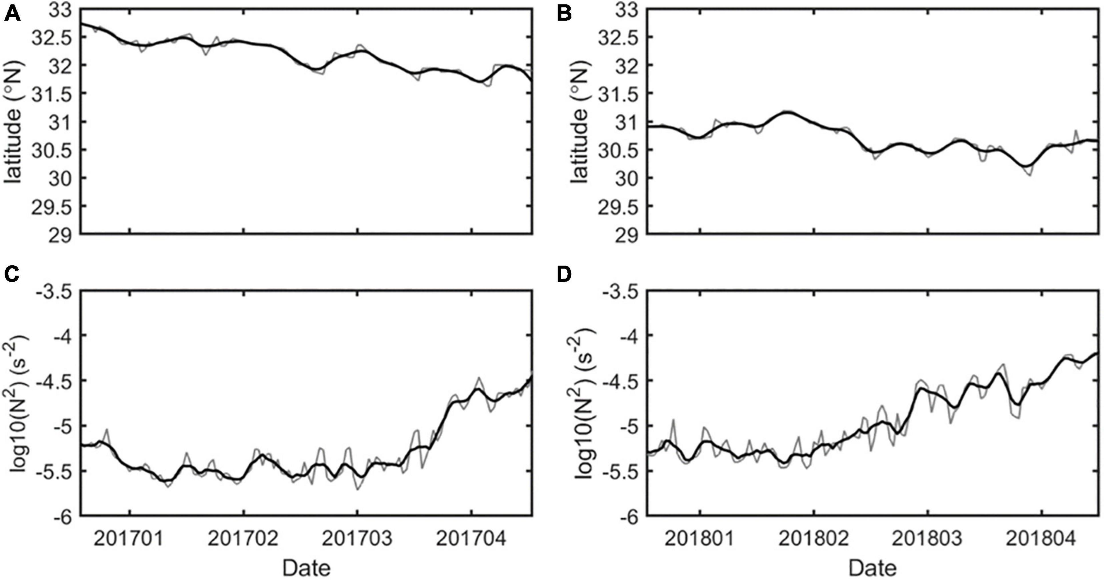
Figure 13. Time series of the main axis of Kuroshio in its southernmost position and regionally averaged (132°−140°E and 28°−35°N) log10 transformed Brunt-Vaisala frequency squared in 2017 (A,C) and 2018 (B,D). The black lines represent 10-day smoothed curves.
To summarize the two processes associated with the SSAE described above, we have attempted to briefly analyze the mechanism by which wintertime CHL aggregates at depths far below the ZEU. The central downward displaced isopycnals caused by the intensified SSAE, and winter mixing deepened to the nutricline due to the thicker MLD and weaker stratification that occurred in winter 2017 (the NLM path period) (Figure 14A). The combined result of these two processes may lead to numerous nutrients and CHL enrichments in the mixed layer, thus generating a CHL bloom in the following April. However, although the SSAE intensified, the shallower MLD and stronger stratification in winter 2018 (the LM path period) limited the depth of downward displacement of isopycnals.
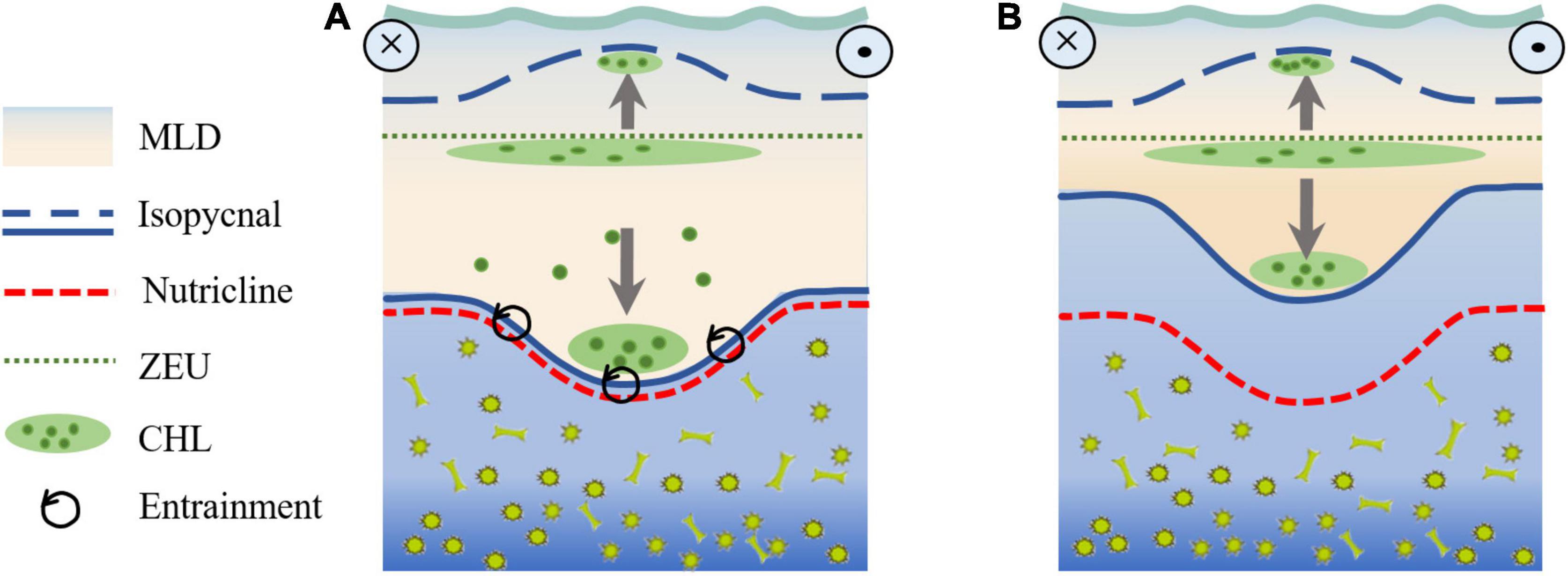
Figure 14. A schematic diagram of SSAE intensification-induced pumping and winter mixing for the (A) NLM and (B) LM paths in the region off the southern coast of Japan.
Summary and Discussion
A long-standing anticyclonic eddy was detected from SLA images with an average radius of approximately 130 km and an average amplitude of 25 cm; this eddy was located at around 30°−32°N, 134°−136°E off Shikoku. With the development of the LM path, the radius, amplitude, and intensity of the anticyclonic eddy gradually increased as its position shifted to the southwest. Different from the idea of the self-sustained oscillation mechanism, the enhanced strength of the anticyclonic eddy that resulted from the eddy kinetic energy was provided by a dramatic increased positive BC conversion rate. The composite anomaly structure suggested that this eddy was a subsurface anticyclonic eddy (SSAE), characterized by having the maximum temperature and salinity anomalies core as well as maximum velocity in the subsurface. In addition, there is significant seasonal variation in the central potential density structure of SSAE during the LM period, with a normal concave isopycnal structure observed from January to April and a convex lens structure observed from May to December; this variation may have been related to the subduction of low-PV STMW.
After that, we further investigated the biogeochemical characteristics of the SSAE; the complete knowledge of which is unclear due to the limited availability of temporally continuous biogeochemical parameter profile data. Based on numerical modeling data, the three-dimensional biogeochemical structure of the SSAE and its contributions to the biogeochemical cycles were investigated. Seasonal variation in eddy dynamic structures decisively influenced its biogeochemical structure. In February, DO within the SSAE showed positive anomalies due to the concave of isopycnals, while CHL and nitrate showed positive anomalies rather than the negative anomalies we usually recognized. From May to December, there was a convex lens structure, and the composite structures of CHL, NO3, and DO within the SSAE showed positive anomalies around the depth of SCM (50−80 m), while elevated CHL and DO concentrations and reduced NO3 concentrations were observed along the periphery of the eddy below the depth of SCM, which may be related to wind-current interaction and sub-mesoscale process-associated vortex Rossby waves. Twofold to threefold increase of CHL was detected in the subsurface CHL maximum layers at the core of the SSAE, and this enhancement was related to the injection of nutrients into the ZEU due to winter mixing and the convex of isopycnals.
The unusual event that high CHL concentration and total phytoplankton were found at depths far below the euphotic layer in the winter of 2017 and 2018 was investigated. More pronounced CHL downward displacement below the ZEU (∼90 m) caused by the SSAE reached 320 m in 2017, whereas it reached only 260 m in 2018. We found that the ultimate downward propagation depth closely fitted the MLD in the SSAE, implying that the vertical displacement of CHL may be mainly explained by the variations in the MLD. In 2017, the enhanced ocean heat losses and wind stresses in January and February, and the weaker upper ocean stratification during the preceding warm season allowed a deeper MLD.
It is worth noting that these two downward propagation processes associated with the SSAE in winter 2017 and 2018 were at different periods of the Kuroshio path; the former occurred during the NLM period on the eve of the path transition, while the latter was during the stable LM period. As the stratification was weaker in early 2017, the conditions were favorable for the formation of the LM path; after the formation of the LM path in July 2017, upper ocean stratification during the July–September as stronger results in a shallower MLD in the subsequent winter 2018. In summary, the combined result of these two processes: (1) the central downward displaced isopycnals caused by intensified SSAE, and (2) winter mixing deepened to the nutricline due to the thicker MLD and weaker stratification in winter 2017 (during the NLM path period) may have led to numerous nutrients and CHL enrichments in the mixed layer, thus generating a CHL bloom in the following April. Whereas, although the SSAE intensified, the shallower MLD and stronger stratification in winter 2018 (during the LM path period) limited the depth of downward displacement of isopycnal.
Chang et al. (2019) suggested that the Kuroshio LM was speculated to be connected to the low eel recruitment in 2018 because of its occurrence when there were lower overall catches of glass eels, while there were more glass eel catches in 2017. As we discussed above, the mixed layer in the SSAE deepened to the nutricline in the winter of 2017, leading to numerous nutrients and CHL enrichments throughout the mixed layer and thus generating a CHL bloom in the following April. This process may have been connected to the increased glass eel catches recorded in 2017. Thus, the physical processes associated with the SSAE during the winter preceding the onset of the LM path may have largely affected local phytoplankton blooms and fish catches.
Oxygen is essential for the survival of individual animals, and it also regulates the global cycles of major nutrients as well as carbon. The oxygen content of the ocean and coastal waters has been declining for at least the past half-century, primarily due to human activities that have increased global temperatures and nutrients discharged to coastal waters. These changes have accelerated the consumption of oxygen by microbial respiration, reduced the solubility of oxygen in water, and decreased the oxygen resupply rate from the atmosphere to the ocean interior; these effects have broad biological and ecological consequences (Breitburg and Levin, 2018). But due to the downward displaced isopycnals caused by intensified SSAE and deepened winter mixing, the dissolved oxygen concentration was elevated throughout the upper water column (Figure 12B), causing local dissolved oxygen levels to increase, and it is important for the survival of individual animals and cycles of major nutrients as well as carbon. Consequently, the physical and biogeochemical process of the studied SSAE and its contributions to the biogeochemical cycles should be taken into account in the future research; there is more waiting for us to explore.
Data Availability Statement
Publicly available datasets were analyzed in this study. This data can be found here: ftp.ifremer.fr/ifremer/argo/dac/, https://hermes.acri.fr/index.php, https://www1.kaiho.mlit.go.jp/KANKYO/KAIYO/, and http://marine.copernicus.eu.
Author Contributions
YD conducted the analyses and wrote the manuscript. FY read through the manuscript and provided revisions. QR, FN, and RW participated in the observation data collection and formal analysis. YSL and YT participated in the discussions and improvement of the manuscript. All authors contributed to the article and approved the submitted version.
Funding
This work was supported by the Global Climate Changes and Air-sea Interaction Program (Grant No. GASI-02-PACSTMSspr), NSFC-Shandong Joint Fund for Marine Science Research Centers (Grant No. U1406401), and the National Natural Science Foundation of Shandong Province (Grant No. ZR2020MD057).
Conflict of Interest
The authors declare that the research was conducted in the absence of any commercial or financial relationships that could be construed as a potential conflict of interest.
Publisher’s Note
All claims expressed in this article are solely those of the authors and do not necessarily represent those of their affiliated organizations, or those of the publisher, the editors and the reviewers. Any product that may be evaluated in this article, or claim that may be made by its manufacturer, is not guaranteed or endorsed by the publisher.
Acknowledgments
We would like to thank Yann Drillet, Marc Tressol, Miloud Rached, Matthieu Clavier, David, and Elena from Copernicus Marine Service for assistance in processing the Global Biogeochemical Analysis and Forecast product, which was obtained from the Copernicus Marine Environment Monitoring Service (CMEMS; http://marine.copernicus.eu). We would like to thank China BGC-Argo Project led by Fei Chai at Second Institute of Oceanography and JAMSTEC (Japan Agency for Marine-Earth Science and Technology) project for the BGC-Argo dataset, which were downloaded from the Coriolis GDAC FTP server (ftp://ftp.ifremer.fr/ifremer/argo). The altimeter products are produced by the Ssalto/Duacs and distributed by the AVISO, with support from the CNES. We would also like to thank the two reviewers FZ and XC for their careful reading and for providing very constructive comments that improved the manuscript.
Supplementary Material
The Supplementary Material for this article can be found online at: https://www.frontiersin.org/articles/10.3389/fmars.2021.766544/full#supplementary-material
Footnotes
- ^ ftp.ifremer.fr/ifremer/argo/dac/
- ^ http://marine.copernicus.eu/
- ^ https://www.nemo-ocean.eu/
- ^ https://hermes.acri.fr/index.php
- ^ https://www.nodc.noaa.gov/OC5/woa18/
- ^ https://www1.kaiho.mlit.go.jp/KANKYO/KAIYO/
References
Anderson, G. C. (1969). Subsurface chlorophyll maximun in the Northeast Pacific Ocean. Limnol. Oceanogr. 14:386.
Assassi, C., Morel, Y., Vandermeirsch, F., Chaigneau, A., and Cambra, R. (2016). An index to distinguish surface- and subsurface-intensified vortices from surface observations. J. Phys. Oceanogr. 46, 2529–2552.
Barreto, D., Saravia, R. C., Nagai, T., and Hirata, T. (2021). Phytoplankton increase along the Kuroshio due to the large meander. Front. Mar. Sci. 8:677632. doi: 10.3389/fmars.2021.677632
Barth, A., Beckers, J. M., Troupin, C., Alvera-Azcárate, A., and Vandenbulcke, L. (2014). Divand-1.0: n-dimensional variational data analysis for ocean observations. Geosci. Model Dev. 7, 225–241. doi: 10.5194/gmd-7-225-2014
Bidigare, R. R., Benitez-Nelson, C., Leonard, C. L., Quay, P. D., Parsons, M. L., Foley, D. G., et al. (2003). Influence of a cyclonic eddy on microheterotroph biomass and carbon export in the lee of Hawaii. Geophys. Res. Lett. 30:1318. doi: 10.1029/2002GL016393
Breitburg, D., and Levin, L. A. (2018). Declining oxygen in the global ocean and coastal waters. Science 359:eaam7240. doi: 10.1126/science.aam7240
Campbell, J. (1995). The lognormal distribution as a model for bio-optical variability in the sea. J. Geophys. Res. 100:13.
Chang, Y., Miyazawa, Y., Miller, M. J., and Tsukamoto, K. J. P. O. (2019). Influence of ocean circulation and the Kuroshio large meander on the 2018 Japanese eel recruitment season. PLoS One 14:e0223262. doi: 10.1371/journal.pone.0223262
Chelton, D. B., Gaube, P., Schlax, M. G., Early, J. J., and Samelson, R. M. (2011). The influence of nonlinear mesoscale eddies on near-surface oceanic chlorophyll. Science 334, 328–332. doi: 10.1126/science.1208897
Chen, Y., Chen, H. Y., Lin, I. I., Lee, M. A., and Chang, J. (2007). Effects of cold eddy on phytoplankton production and assemblages in luzon strait bordering the south china sea. J. Oceanogr. 63, 671–683.
Chiswell, S. M., Calil, P. H. R., and Boyd, P. W. (2015). Spring blooms and annual cycles of phytoplankton: a unified perspective. J. Plankton Res. 37, 500–508.
Dawson, H. R., Strutton, P. G., and Gaube, P. (2018). The unusual surface chlorophyll signatures of Southern Ocean eddies. J. Geophys. Res. Oceans 123, 6053–6069. doi: 10.1029/2017jc013628
Donlon, C. J., Martin, M. J., Stark, J. D., Roberts-Jones, J., Fiedler, E., and Wimmer, W. (2012). The Operational Sea Surface Temperatureand Sea Ice Analysis (OSTIA) system. Remote Sens. Environ. 116, 140–158. doi: 10.1016/j.rse.2010.10.017
Dore, J., Letelier, R., Church, M., Lukas, R., and Karl, D. (2008). Summer phytoplankton blooms in the oligotrophic North Pacific Subtropical Gyre: historical perspective and recent observations. Prog. Oceanogr. 76, 2–38.
Dubinsky, Z., and Stambler, N. (2009). Photoacclimation processes in phytoplankton: mechanisms, consequences, and applications. Aquat. Microb. Ecol. 56, 163–176. doi: 10.3354/ame01345
Dufois, F., Hardman-Mountford, N. J., Greenwood, J., Richardson, A. J., Feng, M., Herbette, S., et al. (2014). Impact of eddies on surfacechlorophyll in the South Indian Ocean. J. Geophys. Res. Oceans 119, 8061–8077. doi: 10.1002/2014JC010164
Dufois, F., Hardman-Mountford, N. J., Greenwood, J., Richardson, A. J., Feng, M., and Matear, R. J. (2016). Anticyclonic eddies are more productivethan cyclonic eddies in subtropical gyres because of winter mixing. Sci. Adv. 2, e1600282–e1600282. doi: 10.1126/sciadv.1600282
Early, J., Samelson, R., and Chelton, D. (2011). The evolution and propagation of quasigeostrophic ocean eddies. J. Phys. Oceanogr. 41, 1535–1555. doi: 10.1175/2011jpo4601.1
Falkowski, P. G., Ziemann, D., Kolber, Z., and Bienfang, P. K. (1991). Roleof eddy pumping in enhancing primary production in the ocean. Nature 352, 5–58. doi: 10.1038/352055a0
Fennel, K., and Boss, E. (2003). Subsurface maxima of phytoplankton and chlorophyll: steady-state solutions froma simple model. Limnol. Oceanogr. 48, 1521–1534. doi: 10.4319/lo.2003.48.4.1521
Frenger, I., Muennich, M., and Gruber, N. (2018). Imprint of southern ocean mesoscale eddies on chlorophyll. Biogeosciences 15, 4781–4798. doi: 10.5194/bg-15-4781-2018
Furuya, K. (1990). Subsurface chlorophyll maximum in the tropical and subtropical western pacific ocean: vertical profiles of phytoplankton biomass and its relationship with chlorophyll a and particulate organic carbon. Mar. Biol. 107, 529–539.
Gaube, P., Chelton, D. B., Samelson, R. M., Schlax, M. G., and O’Neill, L. W. (2014). Satellite Observations of Mesoscale Eddy-Induced EkmanPumping. J. Phys. Oceanogr. 45, 104–132. doi: 10.1175/JPO-D-14-0032.1
Gaube, P., Chelton, D., Strutton, P., and Behrenfeld, M. (2013). Satellite observations of chlorophyll, phytoplankton biomass and Ekmanpumping in nonlinear mesoscale eddies. J. Geophys. Res. Oceans 118, 6349–6370. doi: 10.1002/2013JC009027
Gaube, P., McGillicuddy, D. J. Jr., and Moulin, A. J. (2019). Mesoscale eddiesmodulate mixed layer depth globally. Geophys. Res. Lett. 46, 1505–1512. doi: 10.1029/2018GL080006
Gong, X., Shi, J., and Gao, H. W. (2012). Subsurface chlorophyll maximum in ocean: its characteristics and influencing factors. Adv. Earth Sci. 27, 539–548. doi: 10.1098/rsta.2019.0351
Hense, I., and Beckmann, A. J. (2008). Revisiting subsurface chlorophyll and phytoplankton distributions. Deep Sea Res. I Oceanogr. Res. Pap. 55, 1193–1199. doi: 10.1016/j.dsr.2008.04.009
Huang, J., and Xu, F. (2018). Observational Evidence of Subsurface Chlorophyll Response to Mesoscale Eddies in the North Pacific. Geophys. Res. Lett. 45, 8462–8470.
Imawaki, S., Uchida, H., Ichikawa, H., Fukasawa, M., Umatani, S., and ASUKA Group (1997). Time Series of the Kuroshio Transport Derived from Field Observations and Altimetry Data. Rev. Méd. Chil. 126, 15–18.
Iwamaru, H., Kobashi, F., and Iwasaka, N. (2010). Temporal variations of the winter mixed layer south of the kuroshio extension. J. Oceanogr. 66, 147–153. doi: 10.1007/s10872-010-0012-1
Kawabe, M. (1985). Sea level variations at the Izu Islands and typical stable paths of the Kuroshio. J. Oceanogr. Soc. Jpn. 41, 307–326. doi: 10.1007/bf02109238
Kawabe, M. (1995). Variations of current path, velocity, and volume transport of the Kuroshio in relation with the large meander. J. Phys. Oceanogr. 25, 3103–3117. doi: 10.1175/1520-04851995025<3103:VOCPVA<2.0.CO;2
Kiefer, D. A., Olson, R. J., and Holm-Hansen, O. (1976). Another look atthe nitrite and chlorophyll maxima in the central North Pacific. Deep Sea Res. Oceanogr. Abstr. 23, 1199–1208. doi: 10.1016/0011-7471(76)90895-0
Kouketsu, S., Kaneko, H., Okunishi, T., Sasaoka, K., Itoh, S., Inoue, R., et al. (2016). Mesoscale eddy effects on temporal variability of surface chlorophyll a in the kuroshio extension. J. Oceanogr. 72, 439–451.
Kurogi, M., and Akitomo, K. (2006). Effects of stratification on the stable paths of the kuroshio and on their variation. Deep Sea Res. I Oceanogr. Res. Pap. 53, 1564–1577. doi: 10.1016/j.dsr.2006.07.003
Lea, D. J., Mirouze, I., Martin, M. J., King, R. R., Hines, A., Walters, D., et al. (2015). Assessing anew data assimilation system based on the Met Office coupled atmosphere-land-ocean-sea ice model. Mon. Weather Rev. 143, 4678–4694. doi: 10.1175/mwr-d-15-0174.1
Levy, M., Memery, L., and Madec, G. (1998). The onset of a bloom after deep winter convection in the northwestern Mediterranean sea: mesoscale process study with a primitive equation model. J. Mar. Syst. 16, 7–21. doi: 10.1016/s0924-7963(97)00097-3
Lewis, M. R. (2002). “Variability of plankton and plankton processes on themesoscale,” in Phytoplankton Productivity-Carbon Assimilation in Marine and FreshwaterEcosystems, eds P. J. le, B. Williams, D. N. Thomas, and C. S. Reynolds (Oxford: Blackwell Science), 141–155. doi: 10.1002/9780470995204.ch6
Li, R., Zhang, Z. W., and Wu, L. X. (2014). High-resolution modeling study of the Kuroshio path variations south of Japan. Adv. Atmos. Sci. 31, 1233–1244. doi: 10.1007/s00376-014-3230-4
Lin, I., Lien, C., Wu, C., Wong, G., Huang, C., and Chiang, T. (2010). Enhanced primary production in the oligotrophic South China Sea by eddy injection in spring. Geophys. Res. Lett. 37:L16602.
Lorenz, E. N. (1955). Available potential energy and the maintenance of the general circulation. Tellus 7, 157–167. doi: 10.3402/tellusa.v7i2.8796
Lorenz, E. N. (1960). Energy and numerical weather prediction. Tellus 12, 364–373. doi: 10.1111/j.2153-3490.1960.tb01323.x
Mahadevan, A., Thomas, L. N., and Tandon, A. (2008). Comments on “Eddy/wind interactions stimulate extraordinary mid-ocean planktonblooms,”. Science 320:448. doi: 10.1126/science.1152111
Martin, A., and Richards, K. (2001). Mechanisms for vertical nutrient transport within a North Atlantic mesoscale eddy. Deep Sea Res. II 48, 757–773.
Masuda, S., and Akitomo, K. (2000). Effects of stratification and bottomtopography on the Kuroshio path variation south of Japan. Part II: path transitions in a multiple equilibrium regime. J. Phys. Oceanogr. 30, 1431–1449. doi: 10.1175/1520-0485(2000)030<1431:eosabt>2.0.co;2
McGillicuddy, D. J., Anderson, L. A., Bates, N. R., Bibby, T. S., and Buesseler, K. O. (2007). Eddy/Wind Interactions Stimulate Extraordinary Mid-Ocean Plankton Blooms. Science 316, 1021–1026. doi: 10.1126/science.1136256
McGillicuddy, D. J., Johnson, R., Siegel, D. A., Michaels, A. F., Bates, N. R., and Knap, A. H. (1999). Mesoscale variations of biogeochemical properties in the Sargasso Sea. J. Geophys. Res. 104, 13381–13394. doi: 10.1029/1999JC900021
McGillicuddy, D. J., Robinson, A. R., Siegel, D. A., Jannasch, H. W., Johnson, R., Dickey, T. D., et al. (1998). Influence of mesoscale eddies on new production in the Sargasso Sea. Nature 394, 263–266. doi: 10.1038/28367
Mignot, A., Claustre, H., D’Ortenzio, F., Xing, X., Poteau, A., and Ras, J. (2011). From the shape of the vertical profile of in vivo fluorescence to chlorophyll-a concentration. Biogeosciences 8, 2391–2406. doi: 10.5194/bg-8-2391-2011
Mitsudera, H., Waseda, T., Yoshikawa, Y., and Taguchi, B. (2001). Anticyclonic eddies and Kuroshio meander formation. Geophys. Res. Lett. 28, 2025–2028. doi: 10.1029/2000gl012668
Morel, A., Huot, Y., Bernard Gentili, P., Werdell, J., Hooker, S. B., et al. (2007). Examining the consistency of products derived from various ocean color sensors in open ocean (Case 1) waters in the perspective of a multi-sensor approach. Remote Sens. Environ. 111, 69–88. doi: 10.1016/j.rse.2007.03.012
Morel, Y., and Thomas, L. (2009). Ekman drift and vortical structures. Ocean Model. 27, 185–197. doi: 10.1016/j.ocemod.2009.01.002
Nagano, A., Yamashita, Y., Ariyoshi, K., Hasegawa, T., Matsumoto, H., and Shinohara, M. (2021). Seafloor Pressure Change Excited at the Northwest Corner of the Shikoku Basin by the Formation of the Kuroshio Large-Meander in September 2017. Front. Earth Sci. 8:583481. doi: 10.3389/feart.2020.583481
Nan, F., Yu, F., Wei, C., Ren, Q., and Fan, C. (2017). Observations of an Extra-Large Subsurface Anticyclonic Eddy in the Northwestern Pacific Subtropical Gyre. J. Mar. Sci. Res. Dev. 7:235. doi: 10.4172/2155-9910.1000235
Nencioli, F., Dong, C., Dickey, T., Washburna, L., and McWilliams, J. C. (2010). Vector geometry-based eddy detection algorithm and its application to a high-resolution numerical model product and high-frequency radar surface velocities in the Southern California Bight. J. Atmos Ocean Tech. 27, 564–579. doi: 10.1175/2009jtecho725.1
Qiu, B., and Chen, S. (2006). Decadal Variability in the Formation of the North Pacific Subtropical Mode Water: oceanic versus Atmospheric Control. J. Phys. Oceanogr. 36, 559–568.
Qiu, B., and Miao, W. F. (2000). Kuroshio path variations south ofJapan: bimodality as a self-sustained internal oscillation. J. Phys. Oceanogr. 30, 2124–2137. doi: 10.1175/1520-0485(2000)030<2124:kpvsoj>2.0.co;2
Qiu, G., Wang, H., and Xing, X. (2018). Application of BGC-Argo Floats Observation to Ocean Biogeochemistry. J. Xiamen Univ. 57, 827–840.
Radenac, M. H., and Rodier, M. (1996). Nitrate and chlorophyll distributions in relation to thermohaline and current structures in the western tropical Pacific during 1985–1989. Deep Sea Res. II 43, 725–752.
Rhines, P. B. (2001). “Mesoscale Eddies,”in Encyclopedia of Ocean Sciences, Ed. J. H. Steele (Oxford: Academic Press), 1717–1730.
Rio, M.-H., Pascual, A., Poulain, P.-M., Menna, M., Barceló, B., and Tintoré, J. (2014). Computation of a new mean dynamic topography for the Mediterranean Sea from model outputs, altimeter measurements and oceanographic in situ data. Ocean Sci. 10, 731–744. doi: 10.5194/os-10-731-2014
Rodriguez, F., Varela, M., Fernandez, E., and Zapata, M. (2003). Phytoplankton and pigment distributions in an anticyclonic slope water oceanic eddy (SWODDY) in the southernBay of Biscay. Mar. Biol. 143, 995–1011.
Sasai, Y., Richards, K. J., Ishida, A., and Sasaki, H. (2010). Effects of cyclonic mesoscale eddies on the marine ecosystem in the kuroshio extension region using an eddy-resolving coupled physical-biological model. Ocean Dyn. 60, 693–704. doi: 10.1007/s10236-010-0264-8
Siegel, D., McGillicuddy, D., and Fields, E. (1999). Mesoscale eddies, satellite altimetry, and new production in the Sargasso Sea. J. Geophys. Res. 104, 13359–13379. doi: 10.1029/1999jc900051
Song, H., Long, M. C., Gaube, P., Frenger, I, Marshall, J., and McGillicuddy, D. J. Jr. (2018). Seasonal variation in the correlation between anomalies of sea level and chlorophyll in the Antarctic Circumpolar Current. Geophys. Res. Lett. 45, 5011–5019. doi: 10.1029/2017gl076246
Souza, J., De, B., and Le, T. (2011). Comparison between three implementations of automatic identification algorithms for the quantification and characterization of mesoscale eddies in the South Atlantic Ocean. Ocean Sci. 7, 317–334. doi: 10.5194/os-7-317-2011
Stern, M. (1965). Interaction of a uniform wind stress with a geostrophicvortex. Deep Sea Res. Oceanogr. Abstr. 12, 355–367. doi: 10.1016/0011-7471(65)90007-0
Sugimoto, S., and Hanawa, K. (2014). Influence of Kuroshio Path Variation South of Japan on Formation of Subtropical Mode Water. J. Phys. Oceanogr. 44, 1065–1077. doi: 10.1175/jpo-d-13-0114.1
Sugimoto, T., Ishimaru, T., and Kobayashi, M. (1986). Circulation and water exchange in the anticyclonic gyre off shikoku. Deep Sea Res. A Oceanogr. Res. Pap. 33, 1641–1652.
Sweeney, E. N., McGillicuddy, D. J., and Buesselerd Ken, O. (2003). Biogeochemical impacts due to mesoscale eddy activity in the sargasso sea as measured at the bermuda atlantic time-series study (bats). Deep Sea Res. II Top. Stud. Oceanogr. 50, 3017–3039. doi: 10.1016/j.dsr2.2003.07.008
Taft, B. (1972). “Characteristics of the flow of the Kuroshio south of Japan,” in Kuroshio-its physical aspects, eds H. Stommel and K. Yoshida (Tokyo: University of Tokyo Press), 165–216.
Tsujino, H., Usui, N., and Nakano, H. (2006). Dynamics of Kuroshiopath variations in a high-resolution general circulation model.J. Geophys. Res. 111:C11001. doi: 10.1029/2005JC003118
Winn, C. D., Campbell, L., Christian, J. R., Hebel, D. V., Dore, J. E., Fujieki, L., et al. (1995). Seasonal variability in the phytoplankton community of the NorthPacific Subtropical Gyre. Global Biogeochem. Cy. 9, 605–620. doi: 10.1029/95gb02149
Xing, X., Wells, M. L., Chen, S., Lin, S., and Chai, F. (2020). Enhanced winter carbon export observed by BGC-Argo in the Northwest Pacific Ocean. Geophys. Res. Lett. 47:e2020GL089847. doi: 10.1029/2020GL089847
Xiu, P., and Chai, F. (2011). Modeled biogeochemical responses to mesoscale eddies in the South China Sea, J. Geophys. Res. 116:C10006. doi: 10.1029/2010JC006800
Xiu, P., and Chai, F. (2020). Eddies affect subsurface phytoplankton and oxygen distributions in the North Pacific Subtropical Gyre. Geophys. Res. Lett. 47:e2020GL087037. doi: 10.1029/2020gl087037
Xiu, P., Palacz, A., Chai, F., Roy, E. G., and Wells, M. L. (2011). Iron fluxinduced by Haida eddies in the Gulf of Alaska. Geophys. Res. Lett. 38:L13607. doi: 10.1029/2011GL047946
Xu, G., Dong, C., Liu, Y., Gaube, P., and Yang, J. (2019). Chlorophyll rings around ocean eddies in the north pacific. Sci. Rep. 9:2056. doi: 10.1038/s41598-018-38457-8
Yoon, J.-H., and Yasuda, I. (1987). Dynamics of the Kuroshio largemeander: two-layer model. J. Phys. Oceanogr. 17, 66–81.
Yoshida, S. (1964). A note on the variations of the Kuroshio during recent years. Bull. Japan. Soc. Fish. Oceanogr. 5, 66–69.
Zhang, Z., and Qiu, B. (2020). Surface Chlorophyll Enhancement in Mesoscale Eddies by Submesoscale Spiral Bands. Geophys. Res. Lett. 47:e2020GL088820.
Zhang, Z., Qiu, B., Klein, P., and Travis, S. (2019). The influence of geostrophic strain on oceanic ageostrophic motion and surface chlorophyll. Nat. Commun. 10:2838. doi: 10.1038/s41467-019-10883-w
Keywords: subsurface anticyclonic eddy, physical-biogeochemical structure, chlorophyll, winter mixing, Kuroshio path
Citation: Ding YN, Yu F, Ren Q, Nan F, Wang R, Liu Y and Tang Y (2022) The Physical-Biogeochemical Responses to a Subsurface Anticyclonic Eddy in the Northwest Pacific. Front. Mar. Sci. 8:766544. doi: 10.3389/fmars.2021.766544
Received: 29 August 2021; Accepted: 06 December 2021;
Published: 27 January 2022.
Edited by:
Ying Wu, East China Normal University, ChinaReviewed by:
Feng Zhou, Ministry of Natural Resources, ChinaXavier Carton, Université de Bretagne Occidentale, France
Copyright © 2022 Ding, Yu, Ren, Nan, Wang, Liu and Tang. This is an open-access article distributed under the terms of the Creative Commons Attribution License (CC BY). The use, distribution or reproduction in other forums is permitted, provided the original author(s) and the copyright owner(s) are credited and that the original publication in this journal is cited, in accordance with accepted academic practice. No use, distribution or reproduction is permitted which does not comply with these terms.
*Correspondence: Fei Yu, yuf@qdio.ac.cn