Deep Learning Detection and Recognition of Spot Elevations on Historical Topographic Maps

Introduction

Spot elevations were depicted on historical maps to improve the reader’s interpretation of the terrain, assist the terrain representation shown by contours, indicate points of interest, and, in the case of those at summits and passes, assist aviators when navigating, and are not depicted on modern (digital) vectorized topographic maps in the United States today (Arundel and Sinha 2020). To remedy this absence, research on spot elevations/heights has concentrated on automating techniques to choose appropriate features from the myriad of elevational peaks for cartographic display on topographic maps because their manual selection and generalization is both expensive and time consuming (Baella et al., 2007; Palomar-Vázquez and Pardo-Pascual 2008). However, this research has, in general, been neglected relative to other automated terrain mapping issues such as those in geomorphometry and hydrology (Guilbert et al., 2014).

Methods that extract spot heights from any digital elevation models include simple peak extraction methods devised by Peucker and Douglas (1975), which unconditionally identify all points on a surface with a minimal or maximal extreme. Wood (2004) developed the relative drop method to reduce the maximal points for automated spot height labelling by identifying significant eminences (peaks). Further work by Baella et al. (2007), Palomar-Vázquez and Pardo-Pascual (2008), Chaudhry and Mackaness (2008), Deng and Wilson (2008), Jaara and Lecordix (2011), and Rocca et al. (2017) continued the effort to select salient - or significant - features for spot height display.

Working under the assumption that salient features are those that people name, Arundel and Sinha (2020) chose Geographic Names Information System (GNIS) summit features to address this problem, improving automated spot height calculation for the United States. In conducting this work, they discovered that the best ground-truth source for determining the accuracy of spot height elevations was that depicted in text on the HTMC. This finding prompted the research reported here to detect and recognize spot elevations and recognize their elevation values.

Background

Historical topographic maps contain a plethora of information about the world, some of which is difficult to capture digitally. One complex task is capturing the knowledge contained mainly in text labels, such as natural feature extents and their spatial relationships to other features, and spot elevation values, their representative features, and those features’ locations. The U.S. Geological Survey’s (USGS) historical topographic map collection (HTMC) is no exception. Some themes, such as elevation, hydrography, and geographic names were captured as digital spatial vector databases during the digital revolution and displayed over national imagery to create the USGS’s US Topo product (https://www.usgs.gov/core-science-systems/national-geospatial-program/us-topo). The remainder of the non-digitized embedded data, including spot elevations, is available only collectively as scanned raster images and is not available in machine-readable form (Arundel et al., 2020). Because manual digitization today can be labour and cost prohibitive, automated methods are needed to capture additional features. Extracting specific features from topographic maps not captured as theme geodatabases is a challenging, enduring effort (Pezeshk 2011; Ganpatrao and Ghosh 2014; Arundel et al., 2020; Li et al., 2020; Shbita et al., 2020).

Although most spot elevations were collected at regular intervals in the field for contour construction on historical topographic maps, some were selected to represent distinct map features such as saddles and summits, improving the general perception of the terrain (Thompson 1979). To automate topographic map production in the United States, the digital vector datasets derived from the HTMC are displayed over national imagery to create the USGS US Topo product (https://www.usgs.gov/core-science-systems/national-geospatial-program/us-topo). Non-digitized data are missing from the US Topo, including spot elevations (Arundel and Sinha 2020). The development of a national database of accurate elevations for mountain summits, for example, is important to national mapping, the aviation and recreation industries, geomorphologists, geologists, and other scientists interested in terrain processes and mapping. To address this need, automated workflows that can detect and interpret map text were explored. Automatic classification of text within cartographic contexts can be extended beyond just spot elevation values. A sufficiently trained model could be capable of identifying and cataloguing arbitrary categories of map text, such as geographic feature names, coordinate markings, and other topographic symbology. Generalized interpretation techniques may be used on collections of historical maps other than the HTMC, and have the potential to enable fast, reliable, and thorough data collection from an abundance of historical cartographic sources.

This paper reports progress toward using deep learning optical character recognition (OCR) to detect and recognize spot elevations on USGS historical topographic map images and discusses how this technology can be further applied to extract other information from map content. We describe the implementation and use of the state-of-the-art deep learning OCR architecture called Mask TextSpotter to detect and recognize text on HTMC images. As a proof of concept, our solution focuses on recognition of only single-feature spot elevations, with the future goal of expanding interpretation capability to multi-feature examples of a wide variety of content. Important driving motivations of this research are to ascertain the benefits of utilizing various custom training datasets and parameter configurations in spot elevation text recognition, and to assess the practicality of a generalized technique for text interpretation in historical map contexts.

Optical character recognition, as a field of research in information science, pattern recognition, artificial intelligence (AI), and computer vision, is the translation of digital (raster) images of text into computer-readable text characters. OCR is founded on early technological advances during the first World War, such as image scanners and text-to-speech machines to interpret braille and quickly encode and decode telegraphs (Andersson 1969). OCR technology developed alongside computers, and major systems were operational and available by the 1970s (Stevens 1970; Andersson 1971). Research to improve OCR, particularly in its application across languages, exploded in the 1980s, leading to the release of tools for common use on the web in the early 2000s (Asif et al., 2014). By this time, image processing and pattern recognition techniques had been effectively combined with AI to develop complex OCR algorithms (Chaudhuri et al., 2017). These algorithms, when using ‘big’ input data, require considerable computing capacity. Modern methodologies such as artificial neural networks, deep learning, hidden Markov models, fuzzy set reasoning, and natural language processing have improved recognition to new levels of accuracy (Chaudhuri et al., 2017).

The general steps to accomplish character detection and recognition can be summarized as isolating or locating the text within the image (segmentation), extracting the boundaries of the text itself based on specific patterns (feature extraction), and determining what the extracted text says (classification) (Chen et al., 2021). Challenges when implementing this approach include resolution of touching characters while linking those that are disjointed, distinguishing characters against noisy backgrounds, and distinguishing text from overlapping non-text graphics (Long et al., 2021).

The use of deep learning has recently improved OCR results, particularly in natural scene text recognition, where natural scenes reference images often are available through social media obtained at random places and locations, with differing structures and various backgrounds (Gupta et al., 2016; Gómez and Karatzas 2017). These images are created ‘in the wild,’ and the systems that translate them are generally termed PhotoOCR (Chen et al., 2021; Long et al., 2021). PhotoOCR appears to have the most potential for topographic map text translation due to the size and variability of the available training data. However, text recognition in scanned maps has unique challenges relative to that of photographic images, including scan quality, font differences, feature overlap, and text orientation (Chiang and Knoblock 2010). Current methods focus on solving these obstacles (Chiang et al., 2020; Li et al., 2020; Uhl et al., 2020).

Code bases have traditionally approached the two problems of text detection and recognition separately. For example, single-shot detectors (Wang et al., 2019) or models based on semantic connections within text (Jiang et al., 2021) have been shown to produce good results with specific text types. However, end-to-end code repositories such as TextFuseNet (Ye et al., 2020), which uses a multi-path feature fusion architecture, and Mask TextSpotter (MTS), which is an end-to-end PyTorch code repository, have recently emerged that tie the two tasks together. For this study, we used MTS, which implements a trainable neural network for spotting text with arbitrary shapes (Lyu et al., 2018; Liao et al., 2020). MTS is based on Mask R-CNN, which extends Faster R-CNN by adding a branch that computes the object mask prediction in parallel with the existing branch for bounding box recognition (He et al., 2020). Although most arbitrary-shape scene text spotters use region proposal networks (RPN), which require manually derived anchors to propose text regions, MTS implements a segmentation proposal network (SPN), which functions without anchors.

A practice of the AI community is to develop benchmark datasets against which others may test models and model improvements. Our experiments included the use of five benchmark OCR datasets: Synthtext (Gupta et al., 2016), the challenge datasets from the International Conference on Document Analysis and Recognition (ICDAR) 2013 (https://iapr.org/archives/icdar2013/index.html) and 2015 (https://iapr.org/archives/icdar2015/index.html), TotalText (Ch’Ng and Chan 2017), and SCUT-CTW1500 (SCUT) (Liu et al., 2017).

Methodology

The most current PyTorch implementation of MTS was cloned from GitHub (https://github.com/MhLiao/MaskTextSpotterV3) into a dedicated Anaconda development environment, as suggested by the developer. Our environment setup was originally based on Version 2 of MTS but upgraded upon the release of V3. Customization required modification of the code base to run on a Linux Ubuntu 7.5 server with 128 GB ram, 64 CPUs, 1 NVDIA Tesla P40 GPU with 3840 cores, and with our custom training dataset.

The backbone of Mask TextSpotter V3 is ResNet-50 (He et al., 2016). Proposals are generated by an SPN (Table 1) (Liao et al., 2020), as opposed to the Mask TextSpotter V2 RPN). The SPN provides polygonal (rather than rectangular) representations for the proposals, meaning that the curving or other unaligned features are better detected. A region of interest (ROI) is used instead of RPN to better locate features of interest, and then the SPN proposals are refined by a Fast R-CNN module (Girshick 2015). More accurate detection is realized through the text instance segmentation module (delineating words), and then a character segmentation module (separating individual characters). Finally, text recognition is provided through a spatial attentional module (Figure 1).

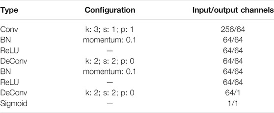
TABLE 1. SPN segmentation prediction module details. “Conv”: convolution operator; “BN”: batch normalization; “DeConv”: de-convolution operator; “k”: kernel size; “s”: stride; “p": padding (recreated following).

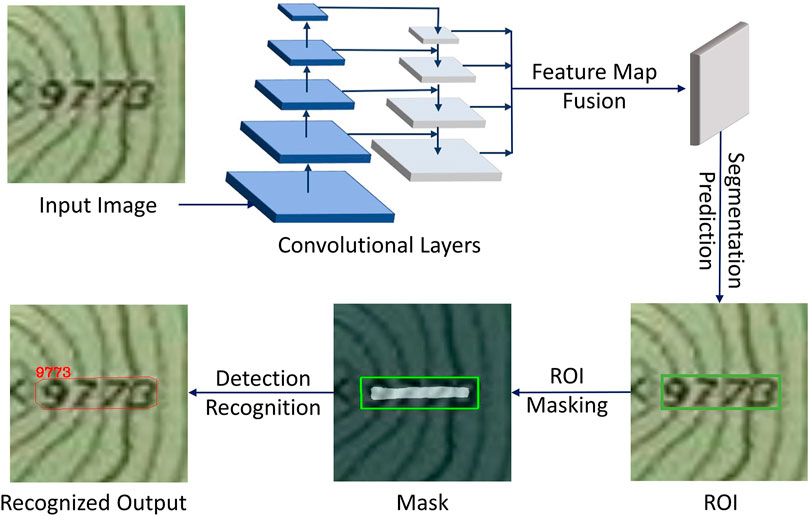
FIGURE 1. Mask TextSpotter V3 workflow starting with input image, which is convolved through multiple layers to produce feature maps. Feature maps are fused, segmented, masked, and the text characters recognized.

The MTS repository includes a link to a serialized benchmark PyTorch model (.pth file), pretrained with the Synthtext dataset. This pre-trained model can be used to initialize the learnable parameters of new models, which can then be further finetune trained with some set of benchmark or custom data, or a mix of both. Utilizing pre-trained weights reduces the training time needed to achieve high performance and allows finetuning parameters with relatively small datasets. This method was used in all experiments.

The learning workflow begins with acquisition of the base data, from which training image/label pairs are created. All training data (including benchmark datasets) are randomly subdivided into training and testing) sets, which are then input to the MTS workflow. The downloaded pretrained (on Synthtext) model is finetuned using the training set, and then used to predict the labels of the testing set. Inferences are evaluated against the ground truth labels and statistics are generated using common machine learning metrics (Figure 2).

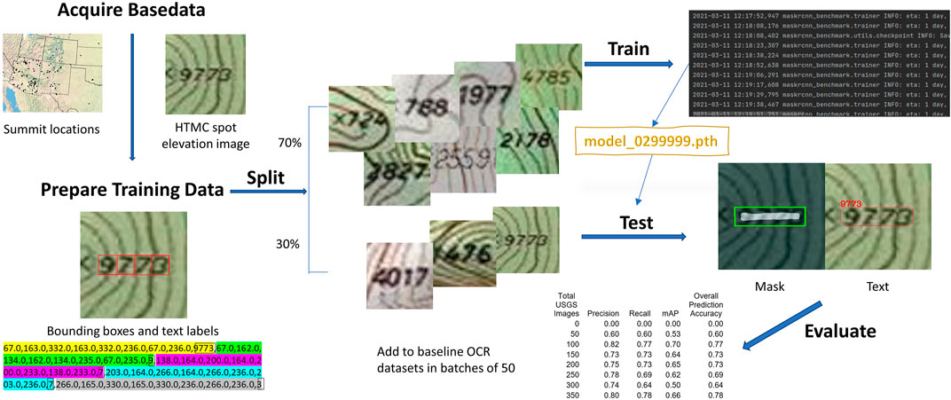
FIGURE 2. A step-by-step overview of the spot elevation detection and recognition learning workflow.

During the custom training data preparation phase, GNIS summits were randomly selected across the coterminous United States (Figure 3). Bounding boxes for each selected point’s spot elevation were heads-up digitized in a geographic information system (GIS) as a vector shapefile using an HTMC service for reference (https://services.arcgisonline.com/ArcGIS/rest/services/USA_Topo_Maps/MapServer). Boxes were placed around the full text of the elevation values displayed on the HTMC, as well as each individual numeric character within that bounding box (Figure 4). The bounding coordinates and elevation values themselves were added to the shapefile for later use.

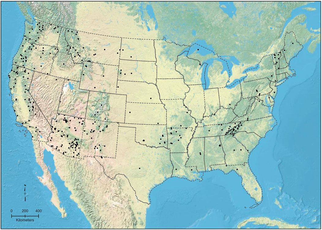
FIGURE 3. Distribution of spot elevations analyzed in the study.

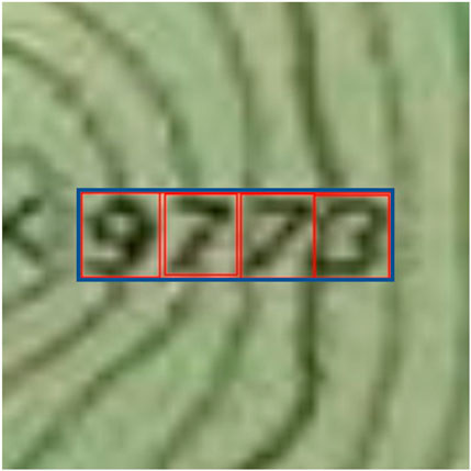
FIGURE 4. A training image of the HTMC showing bounding boxes for the spot elevation 9773. The blue box is the outer bounding area, and each red box delimits a single digit. Bounding boxes are represented to the machine via text labels rather than displayed on the image as seen here.

To obtain images of each spot elevation in the historical maps, we developed code to automatically calculate the geographical extent of an area surrounding each manually digitized spot elevation, then request and download the corresponding image from the HTMC service. To determine the image extent to request, the geographic bounding coordinates of each feature are retrieved from the previously prepared shapefile, then a scalar is applied to the coordinates in every cardinal direction to form an extent that included a small area around the elevation text. Each image is downloaded at a map scale of 1:4,000 with image dimensions of 400 × 400 pixels and centered on the bounding box of its spot elevation marking. Additionally, each image contains only a single spot elevation so that we may isolate these features in experimentation.

Creation of label files from digitized bounding boxes is automated to extract, format, and record bounding box coordinates for each spot elevation. The bounds of the text features are gathered from the shapefile, stretched to be perfectly rectangular, and converted from geographical to pixel coordinates. Pixel coordinates are relative to the origin (0,0), which is located at the upper left corner of the image. The pixel coordinates and their corresponding elevation value are then written to a text file in the transcription format required by MTS to create the image label (Figure 5). This is the same format used by benchmark datasets. The label creation process was completed for each of the selected spot elevations through code. The resulting HTMC spot elevations dataset (referred to as the custom USGS dataset) contained 353 image/label pairs, which was reduced to 350 by randomly removing 3 examples. This was done to create a round, divisible number for training/testing split, and for incremental additions to training sets. Elevation values chosen to display are in integer feet and range from 2 to 5 digits in length. Corresponding values range from 26 (meters) to 12,632, with a mean of 4328 and standard deviation of 2585.

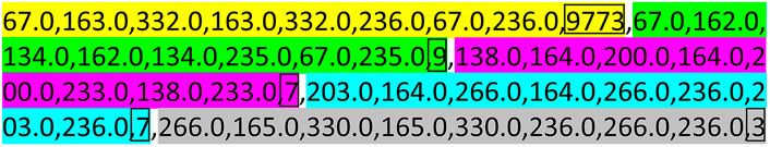
FIGURE 5. Transcription format of the label text file spotElev_Num201. txt, which corresponds to the image shown in Figure 4. The first set (yellow) represents the outer bounding box (xmin, ymin; xmax, ymin; xmax, ymax; xmin, ymax) and the full elevation value (9773). Subsequent sets (green, pink, blue, gray) denote the bounding boxes and content of each character, in the same format.

Advanced experiments used augmented datasets along with the original custom image/label pairs used in initial tests. Data augmentation is the process of increasing the volume of custom data by creating slightly modified copies of existing data (Shorten and Khoshgoftaar 2019). This allows for the creation of substantially larger and more diverse datasets, which in turn leads to more robust predictive models.

Augmentation includes various manipulations that can be applied one at a time, or several can be combined in a single example. For each individual or combined augmentation that is applied, the number of custom examples can be increased by a factor of up to 2, excluding images in which the example becomes invalid. For the USGS custom dataset, invalid images included those where the spot elevation text is unrecognizable or cut off by an edge of the image, or where multiple spot elevation features are present in the same image. Augmentation types in the USGS set include feature frame offset (translation), varying image scale, and varying image rotation. Using a method similar to that of the original set, spot elevation images and labels are automatically retrieved and formatted, with the added options to apply any of the listed augmentation types (Figure 6). As it is not clear yet as to how the operational testing data will be exposed to the trained model, various potential augmentations were chosen.

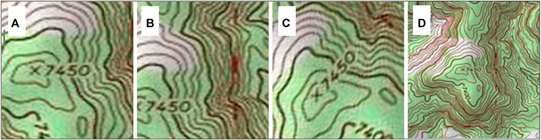
FIGURE 6. Examples of each augmentation type for spotElev_Num84: (A) original centred, (B) offset 0.001° NE in latitude and longitude, (C) rotated 48° counterclockwise, and (D) scaled at 1:12,000.

Frame offset is applied before an image is downloaded by adding a small positive or negative change in both the latitude and longitude of the requested image extent. The offset values are randomly generated within a range that is calculated based on the original extent of the feature such that no offset will result in spot elevation values that are cut off beyond the bounds of the 400 × 400 pixel image.

Variable scales are created in a similar manner. The HTMC request endpoint includes a parameter to adjust the scale of a downloaded image—the user need only pass in a value to retrieve the image at that scale. Scale values are randomly generated between 20,00 and 16,000. These values were chosen in consideration of feature truncation at low scales and conversely, feature readability at high scales. This augmentation type also has the added complexity of handling multi-feature images. Our study uses only single-feature examples for precise experimentation but applying a high scale to a feature sometimes leads to the inclusion of other spot elevations in the same image. We manually sorted through every scale-augmented example and removed those with multiple visible spot elevations.

In contrast to frame offset and scale augmentations, which are both pre-download processes, rotation is implemented post-download. After the original image extent is retrieved and its corresponding label is formatted, a rotation function is applied to the image and label separately. This function modifies the image and label based on a random counterclockwise rotation angle between 0 and 90°, including 0 but not 90. This range was chosen to reflect the same range for rotation augmentations in the MTS V3 paper (Liao et al., 2020).

Augmentations of every type were generated for each of the original spot elevations and included in a single dataset along with the original, centered data, giving us access to a much larger and more diverse volume of custom data with which to experiment (Table 2). After removing the few invalid images, each single augmentation set was split at a 70/30 ratio into training and test subsets, respectively. The larger mixed set was created by adding the images and labels from all other training and test sets into respective mixed training and test sets. That way, the mixed test subset is mutually exclusive with the mixed training subset and both subsets also maintain mutual exclusivity across other sets so that no test images from, for example, the scaled set, would be present in the mixed training set. This also ensures that no images from other training sets are present in the mixed test set.

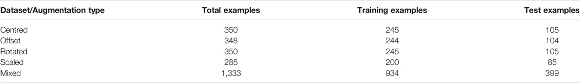
TABLE 2. Example counts for each dataset used in the set of augmentation experiments.

Experiments

Several metrics were used to evaluate the classification results generated by our deep learning workflow (Table 3). Precision describes the proportion of positive identifications that are correct, whereas recall is a measure of the proportion of actual positives identified correctly. Precision and recall results are based on the accuracy of the entire label, as compared to individual characters. The Average Precision mainly considers placement of the predictive bounding boxes relative to the ground-truth, a value that is less important in an operational application. The harmonic mean, in this case, is equivalent to the F-score and provides a single measure of the models’ ability to predict the correct spot elevation value. This metric is commonly used as a measure of accuracy and is often referred to as such. Additionally, the F-score was the primary metric used to analyse individual model performance and compare models against each other.

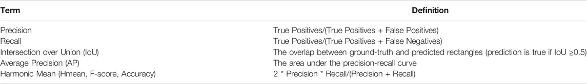
TABLE 3. Metrics/terms used in evaluating the results.

Initial work focused on gathering a baseline performance metric with which to compare other results. We were interested to see if a benchmark-trained deep learning model with the default configuration could recognize text in HTMC images without training on any custom examples. The pretrained model was finetuned with data from the benchmark sets ICDAR 2013, ICDAR 2015, SCUT, and Total Text, then evaluated against the entire USGS dataset. As expected, this test yielded poor performance (Table 4). Without any custom data, the workflow was unable to predict the correct value of any of the labels in the USGS dataset (Table 4, USGS Training Images equals 0).

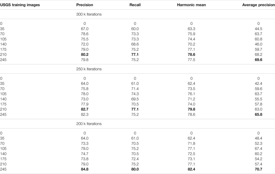
TABLE 4. Metrics describing classification results of detection/recognition workflow by incrementally increasing the number of custom training images by 35, and by decreasing the number of total training iterations by 50 k intervals. Bold text indicates the best performance in the set of tests with that model.

The first set of experiments tested the effect of using various quantities of custom data for finetuning a pre-trained (on Synthtext) PyTorch model. These experiments finetuned the same pretrained model as the baseline but included a mix of benchmark data and custom USGS images. The USGS dataset was weighted at a 0.5 ratio, whereas the supporting datasets (the two ICDAR datasets, SCUT and Total Text) were weighted at 0.1 each. This means the USGS dataset had 5 times the impact of each other individual dataset, and twice the impact of the others combined.

Our custom dataset, containing 350 examples, was split 70% 245) into the training subset and 30% (105) into the testing subset. The test set was the same for all evaluations, but models were trained on sets that incrementally added batches of 35 of the entire 245-image training set, to observe the impact of each additional batch on prediction ability.

This method is less comprehensive than, for example, a K-fold test where each image in the entire dataset is tested exactly once and trained K-1 times, and the average performance is analyzed. However, due to the amount of training time needed to run such a set of experiments, it was more practical to utilize the 70/30 split with the knowledge that the results may not be the best representation of a model’s capability. Still, a single test subset can give us a good estimation of the accuracy of a model, and it is likely that training and testing with other subsets would produce similar outputs.

The base learning rate was set to 0.002 with a weight decay of 0.0001 at a single image per batch for 300,000 iterations. Available server memory limited the number of images per batch. A model checkpoint was saved after every 5,000 iterations. The final model checkpoint was tested at a single image per batch purely on the USGS images from the evaluation set. The model predictions were evaluated against the ground truth labels and interpreted using the previously described performance metrics (Table 4).

Complementary to this set of runs, we conducted experiments to investigate the effect of reducing the number of training iterations. MTS is constructed to run in two phases, pre-training on SynthText (synthetic text) and fineturning on real-world data. By training on top of the SynthText pretrained model, we are essentially using the training dataset as the validation dataset for fineturning, and the testing dataset as inference. Due to this, performance improvements along the epochs must be analyzed for better inferences. Training a single model requires an average of ∼40 h to complete 300 k iterations, which renders the testing of parameter changes costly. Loss during training falls rapidly for the first 50 k iterations and appears to level out around 200 k iterations with no further improvement (Figure 7). We compared results across iterations diminishing at 50 k intervals to understand whether iterations could be reduced to decrease training time without a significant decrease in predictive ability. A set of iterative training runs was computed two more times with the same configurations and datasets except for the number of training iterations reduced to 250,000 and 200,000, respectively (Table 4).

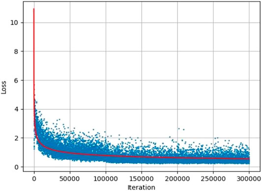
FIGURE 7. Loss by iteration for a training run with 300 k iterations.

The first set of results demonstrates promising detection ability with the addition of only a small number of map-specific training images to the dataset. The addition of just 35 USGS training image/label pairs significantly improved predictive capability—from 0 to 63.3% accuracy (Hmean), and the addition of 210 map-text training images resulted in 78.6% overall accuracy, a 15.3% increase. The highest accuracy across all models in this experiment was produced with 245 training images and 200 k iterations, with Hmean of 82.4%. In general, as the number of USGS training images increases, the Hmean also increases (Figure 8).

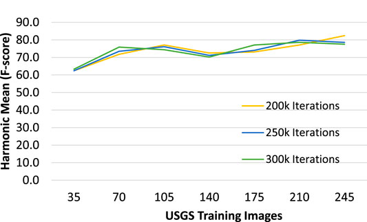
FIGURE 8. Test accuracy by 35-image batches using 200 k, 250 k, and 300 k training iterations.

Training time for 250 k iterations was reduced by 37.5% to 25 h, and training time for 200 k iterations was reduced by 50% to 20 h. Little or no improvement was made in Hmean produced by models with higher iteration counts, which is a strong indicator that 300 k iterations is not the optimal training configuration. It is possible that iteration counts as low as 100 k may produce comparable accuracy and vastly reduce training time.

An interesting pattern is that every model exhibited poorer performance with the 140-image training set than it did with the 105-image set. This is likely due to some error within the 35-image batch that was added to the 105 set. Including that batch in training reduced the model’s general ability to interpret spot elevations, regardless of the number of training iterations. Due to the complex nature of how a model interprets image content, it is not easy to deduce why this particular batch causes a drop in accuracy when included in finetuning. Further investigation would be necessary to draw conclusions.

A similar phenomenon occurred with the addition of a batch to the 210-image set (to make 245 total). However, in this case, the 200 k model did not suffer the decrease in accuracy that the other two did. In fact, it increased the accuracy to the highest recorded for this set of experiments. Yet again the cause of this anomaly is difficult to determine due to the nature of deep learning, and it warrants further investigation.

Advanced experiments made use of data augmentation, which automatically generates new examples for training and testing. Data augmentation includes various ways of manipulating copies of existing data to create similar but distinct new data. This allows for increased volumes of relevant custom training and test examples, which, as indicated by previous experiments, is a good means to achieve higher performance. Data augmentation also provides a greater diversity of examples, which can extend the generalizability of the model.

For this set of tests, we were interested in attaining the highest possible model accuracy, utilizing datasets expanded with augmentations to realize this goal. All models were initialized with the default pretrained model, then finetuned exclusively with USGS training data. The additional benchmark datasets were used to finetune when very little training data were available (starting at 35 images), but then eliminated when the data were increased by augmentation. The base learning rate was set to 0.0002 (10× lower than previous experiments, to avoid divergence in model parameters) with a weight decay of 0.0001 at a single image per batch for 300,000 iterations (both same as before).

To observe the effects of each separate augmentation type when used for training and compare that performance against previous models, we computed a total of 5 finetuned training runs: one for the original centered dataset, one for each augmentation set individually (offset, rotation, and scale), and one for the mixed dataset, composed of all examples from the other sets. The models produced by each training run were evaluated against each test set, 5 for each model (Table 5). Our primary metric for analysis, harmonic mean, was plotted for each output (Figure 9).

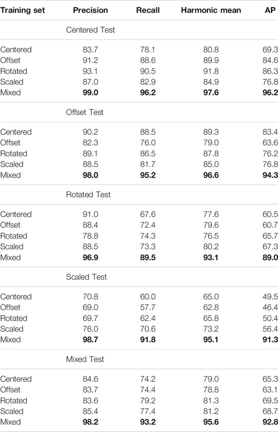
TABLE 5. Evaluation results of models trained with augmented datasets. Each training subset was used to finetune a single model, then each model was evaluated against each test subset for a total of 25 evaluation outputs. Bold text indicates the best performance in the set of tests with that model.

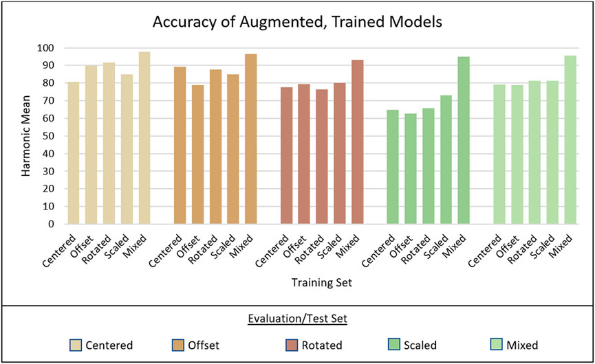
FIGURE 9. Visualization of the harmonic mean (Hmean) for each evaluation output. The bottom axis displays which set the model was trained on and each group of 5 are results from a single evaluation set.

The center-trained model, when evaluated on the centered test dataset, performed similarly to the model trained on the same images for 300 k iterations from the previous experiment set. The center-trained model produced 80.8% Hmean on the 245-image centred evaluation set, and the 300 k model from before achieved 77.5% Hmean (+3.2%). Although there is a slight improvement in the center-trained model, the results are comparable. This was expected because these models used the same dataset of centered spot elevation images and had nearly identical configuration parameters. However, a few differences were noted in the two experiments: the dataset of centered spot elevations was split into different training and evaluation sets for both experiments, the learning rate parameter was 10x lower for the center-trained model, and the 300 k model included benchmark data in its training, whereas the center-trained model used 100% USGS data. Variance in accuracy probably stems from these differences in configuration and dataset split. Further investigation may ascertain more exact explanations and to optimize configurations, although such clarifications are not imperative because the difference is small.

The most noteworthy result from these experiments was that the mix-trained model vastly out-performed all others in every evaluation. We had expected the mixed dataset to generally produce the best results due to its larger training set size and increased training diversity, although the increase in performance was considerably greater than we anticipated. The average Hmean scores across all tests were calculated for each model: center-trained achieved 78.3% average Hmean, offset-trained had 78.0%, rotated-trained had 80.6%, scaled-trained had 80.9%, and mix-trained had 95.6%. The mix-trained model performed 14.7% better than scaled, which has the next highest accuracy. Compared to the four non-mixed models, which had a range of just 2.6% variance between the lowest (centered) and highest (scaled), the mix-trained model greatly improved prediction capability. We can conclude that models trained with mixed-augmentation data are superior to those trained with only a single augmentation method, or none. Further experimentation to determine the most effective types and compositions of augmented data would be beneficial, and implementation of other techniques such as data synthesis may also benefit performance through the creation of even more custom data.

Discussion

Incorrectly predicted image labels in the mixed train/test dataset fall into three general groups: overlapping features, excessive noise, and small map scale. Overlapping features is the most common problem (30% of the errors in the mixed train/mixed test experiment) and refers to other features intersecting the number characters themselves (Figure 10).

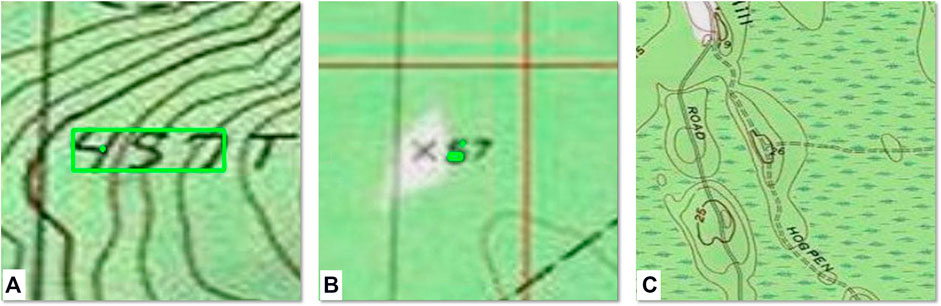
FIGURE 10. Three error types that the study approach failed to resolve, and ROI output from the RNP (A) contours (or other features) overlap/intersect with elevation text (also showing image noise); although the larger ROI is accurate, the prediction was too low to be considered in the character mask process (B) image noise, possibly introduced during the scan process; two small ROIs do not represent the numeric string 57 well, and (C) introduction of too many other features in zoomed out images (also showing overlapping features); no proposals were generated.

Many spot elevations were correctly detected despite overlapping features. Those typically have more even (square or mechanical) text - appearing less like handwriting, thicker line strokes relative to surrounding features, and/or intersection of other lines with fewer characters of the whole elevation string. The combination of the three issues in Figure 10A resulted in no prediction whatsoever, although a good ROI was proposed by the SPN, as well as one small proposal on part of the character 4 (Figure 10A). However, the SPN calculated the likelihood of both ROIs to be true too low to pass to the character mask process. These errors can be reduced through the inclusion in the training dataset of more overlapping strings, particularly with less uniform text.

Several small, poor ROIs were proposed for the noisy image depicting the spot elevation 57 (Figure 10B), and those only vaguely represented the first character 5. The poor quality of the image results in a noisy scene, although to the human eye the characters are easy to identify, and caused 19% of the errors in the mixed/mixed experiment. Noise can be reduced through various filters, which is an area of potential improvement in this work. Some portions of the HTMC exhibit JPEG artifacts, resulting from the way the original JPEG compression and its discrete cosine transform function when too much compression is applied. These artifacts can be fine for interpretation by the human eye but can introduce subtle features that may be confusing to a computer. To reduce these artifacts the image needs to be filtered. Both OpenCV (Bradski 2000) and Scikit-Learn (Pedregosa et al., 2011) have image filters geared towards denoising images and implement non-local means denoising algorithms given by Buades et al. (2011). Scikit-learn also draws from Darbon et al. (2008). The edge-preserving Perona-Malik denoising filter has been used with medical imagery (Halim et al., 2014) and elevation data (Xu et al., 2021). Many studies address JPEG related artifacts and noise (for example, Shohdohji et al., 2002; Popovici and Withers 2007; Chen and Wu 2017). Some studies have analyzed the use of machine learning to address the issue (Chang et al., 2006; Quijas and Fuentes 2014; Zhang et al., 2016). Such an approach could be investigated further to determine applicability.

Another possible cause of poor prediction on this spot elevation may be due to the number of characters. Most spot elevations have three to four characters. In fact, this in part may also contribute to problems identifying the spot elevation 26 in 10C. This issue can be addressed through the addition of more, shorter-stringed spot elevations to the custom training dataset.

In addition to the short string, the image in 10C is scaled out and so contains more conflicting information, including other strings of characters—both alphanumeric and numeric—and various other features types, such as marsh symbols, roads, and trails. It also suffers from overlapping features as the index (bold) contour line runs through the 2 and a lighter contour line “closes” the 6. Scaling issues accounted for 11% of the mixed-mixed errors. Hence, adding more scaled images to the training data would be useful. On the other hand, the spot elevations in many scaled images appearing to have the same characteristics were correctly predicted. The discerning factor in this particular image may be the shortened string of the spot elevation value.

To explain the remaining mixed-mixed errors would require some advanced assessment techniques as they were not obvious from our visual evaluation. However, only 5 images were incorrectly predicted in the mixed-centered experiment. Out of these 5 errors, 4 (80%) were due to overlapping features, and the remaining error was caused by image noise.

The ability to generalize the approach to larger map areas or a map service, as well as to other map text classes, would benefit from additional study. Although the prediction accuracy in the controlled, small images used in this study is quite high, further experiments could expand to less controlled imagery to understand its performance, and what is beneficial to improve accuracy. Because finetuning increased with greater custom data, place name labels were eventually ignored. This behavior is desired in the case where the extraction of only one class of text (in this case, spot elevations) is needed. Further experiments could be used to understand whether this approach is the most beneficial, or whether it is more productive to label and classify all text in training images. Another area of concern for generalizing is to other map products, such as National Geographic or OpenStreetMap, where different font types, text placement, etc., may not be represented in the existing training dataset.

Conclusion

Our experiments demonstrate that deep learning OCR is a viable method for map text interpretation. We achieved high accuracy performance on single feature spot elevation examples within HTMC raster images and this success can likely be extended to additional text instances within the HTMC and other map contexts. The proposed approach could be applied to many map-text detection and recognition projects by incorporating map-specific training examples. This proposal can be tested using other map types, such as other USGS historical maps, OpenStreetMap, or National Geographic maps, and can boost knowledge in engineering, geography, and cartography, particularly through the data mining processes.

Expanding usability to other map types would require the creation of custom image/label pairs that depict various text types within the given map contexts, which is a costly endeavour when done by hand. However, augmentation techniques such as the ones described in this paper could be utilized to reduce the workload needed to craft custom datasets. Additionally, augmentation directly increases the volume of available data to train a model, which generally increases the overall accuracy.

Models have shown to be effective with reduced iteration counts in the training phase. When reduced from the default 300 k iterations to 200 k iterations, there was little or no change in performance. Reducing the number of training iterations can greatly decrease the needed training time, so could be considered in future experiments.

Despite excellent performance when training with the larger mixed dataset, some spot elevation images are still not properly interpreted, or even not detected at all. These problems are difficult to troubleshoot because the machine learning algorithm is essentially a black box. Techniques such as heatmap generation or salient feature detection (Aodha et al., 2019) may be able to provide more insight into why our models are unable to accurately recognize certain spot elevations and possibly lead to an elegant solution to further the capability of future text recognition models.

Other investigative diagnostic tools may be available, and it would be prudent to seek these out or develop custom tools to facilitate the troubleshooting process. Visualization methods may be of use in future production environments and would be invaluable when expanding functionalities or developing new experiments. Potential methods include deconvolution (Zeiler and Fergus 2014), heat maps (Samek et al., 2017), and salient maps (Rashid et al., 2021). Our study is the first application of Mask TextSpotter, as far as we are aware, to historical topographic map text recognition. With an overall word recognition accuracy of ∼95%, the method compares favorably to other studies in historical map text detection and recognition. For example, Weinman et al. (2019) found a 22% word recognition error with their methods that depended on a lexicon, which is useless in the case of numeric strings. Chiang and Knoblock (2010) achieved word recognition recall and precision in the 80% range using their approach to essentially ‘normalize’ the map text to feed into commercial OCR software. Accuracies of our approach are also higher than that reported by (Yu, 2016) that added additional contextual information for the recognition of historical map text. However, these studies seek to recognize alpha and numeric characters, making a direct comparison of the results impossible.

Because the room for improvement in accuracy is small in this limited study, we can look forward to ways this accuracy will plummet in an operational context, and discover enhancements needed to recover it. Thus, such research could focus on the challenges of recreating this performance on a larger spatial scale to develop a spot elevations database. These issues include map tiling methods, detecting multiple features in a single image, handling disjointed text, creating and appending the derivative database, and identifying and removing instance multiples, to name a few. Meeting these challenges would contribute to general machine learning research and specifically text recognition work and forward the goal of deriving a spot elevations database for use by the global community.

Data Availability Statement

The datasets presented in this study can be found in online repositories. The names of the repository/repositories and accession number(s) can be found below: https://osf.io/9pgdf/?view_only = c294460771114afc9ba0253bc2d8fc0d.

Author Contributions

SA and TP contributed to conception and design of the study. PT guided technical progress. SA and TP performed the statistical analysis. SA wrote the first draft of the manuscript. SA, TP, and PT wrote sections of the manuscript. All authors contributed to manuscript revision, read, and approved the submitted version.

Funding

This research was supported in part by the National Science Foundation, Grant No. 1853864.

Conflict of Interest

The authors declare that the research was conducted in the absence of any commercial or financial relationships that could be construed as a potential conflict of interest.

Publisher’s Note

All claims expressed in this article are solely those of the authors and do not necessarily represent those of their affiliated organizations, or those of the publisher, the editors and the reviewers. Any product that may be evaluated in this article, or claim that may be made by its manufacturer, is not guaranteed or endorsed by the publisher.

Acknowledgments

Any use of trade, firm, or product names is for descriptive purposes only and does not imply endorsement by the U.S. Government. This article has been peer reviewed and approved for publication consistent with U.S. Geological Survey Fundamental Science Practices (https://pubs.usgs.gov/circ/1367/).

References

Aodha, O. M., Cole, E., and Perona, P. (2019). “Presence-only Geographical Priors for fine-grained Image Classification,” in Proceedings of the IEEE International Conference on Computer Vision, 2019-Octob, 9595–9605. doi:10.1109/ICCV.2019.00969
Arundel, S. T., Li, W., and Wang, S. (2020). GeoNat v1.0: A Dataset for Natural Feature Mapping with Artificial Intelligence and Supervised Learning. Trans. GIS 24 (3), 556–572. doi:10.1111/tgis.12633
Arundel, S. T., and Sinha, G. (2020). Automated Location Correction and Spot Height Generation for Named Summits in the Coterminous United States. Int. J. Digital Earth 13 (12), 1570–1584. doi:10.1080/17538947.2020.1754936
Asif, A. M. A. M., Hannan, S. A., Perwej, Y., and Vithalrao, M. (2014). An Overview and Applications of Optical Character Recognition. Int. J. Adv. Res. Sci. Eng. 3 (7), 262–274.
Baella, B., Pla, M., Palomar-Vasquez, J., and Pardo-Pascual, J. (2007). Spot Heights Generalization: Deriving the Relief of the Topographic Database of Catalonia at 1:25 000 from the Master Database. Workshop on Generalisation and Multiple Representation, 1–16. Available at: http://aci.ign.fr/BDpubli/moscow2007/Blanca_ICAWorkshop.pdf (Accessed November 2014.
Buades, A., Coll, B., and Morel, J.-M. (2011). Non-Local Means Denoising. Image Process. Line 1, 208–212. doi:10.5201/ipol.2011.bcm_nlm
Ch'ng, C. K., and Chan, C. S. (2017). Total-Text: A Comprehensive Dataset for Scene Text Detection and Recognition. Proc. Int. Conf. Document Anal. Recognition, ICDAR 1, 935–942. doi:10.1109/ICDAR.2017.157
Chang, C.-C., Chan, C.-S., and TsengSen, C.-S. (2006). Removing Blocking Effects Using an Artificial Neural Network. Signal. Process. 86, 2381–2387. doi:10.1016/j.sigpro.2005.11.006
Chaudhry, O. Z., and Mackaness, W. A. (2008). Creating Mountains Out of Mole hills: Automatic Identification of hills and Ranges Using Morphometric Analysis. Trans. GIS 12 (5), 567–589. doi:10.1111/j.1467-9671.2008.01116.x
Chaudhuri, A., Mandaviya, K., Badelia, P., and K Ghosh, S. (2017, Optical Character Recognition Systems for Different Languages with Soft Computing). 248 doi:10.1007/978-3-319-50252-6
Chen, T., and Wu, H. (2017). “Artifact Reduction by Post-Processing in Image Compression,” in Digital Video Image Quality and Perceptual Coding, 459–488. doi:10.1201/978142002782210.1201/9781420027822-15
Chen, X., Jin, L., Zhu, Y., Luo, C., and Wang, T. (2021). Text Recognition in the Wild. ACM Comput. Surv. 54 (2), 1–35. doi:10.1145/3440756
Chiang, Y.-Y., Duan, W., Leyk, S., Uhl, J. H., and Knoblock, C. A. (2020). “Historical Map Applications and Processing Technologies,” in Using Historical Maps in Scientific Studies. SpringerBriefs in Geography (Cham: Springer), 9–36. doi:10.1007/978-3-319-66908-3_2
Darbon, J., Cunha, A., Chan, T. F., Osher, S., and Jensen, G. J. (2008). “Fast Nonlocal Filtering Applied to Electron Cryomicroscopy,” in Proceedings (ISBI), 1331–1334. doi:10.1109/ISBI.2008.4541250
Deng, Y., and Wilson, J. P. (2008). Multi‐scale and Multi‐criteria Mapping of Mountain Peaks as Fuzzy Entities. Int. J. Geographical Inf. Sci. 22 (2), 205–218. doi:10.1080/13658810701405623
Ganpatrao, N. G., and Ghosh, J. K. (2014). Information Extraction from Topographic Map Using Colour and Shape Analysis. Sadhana 39 (5), 1095–1117. doi:10.1007/s12046-014-0270-5
Girshick, R. (2015). “Fast R-CNN,” in Proceedings of the IEEE International Conference on Computer Vision, 2015 Inter, 1440–1448. doi:10.1109/ICCV.2015.169
Gómez, L., and Karatzas, D. (2017). TextProposals: A Text-specific Selective Search Algorithm for Word Spotting in the Wild. Pattern Recognition 70, 60–74. doi:10.1016/j.patcog.2017.04.027
Guilbert, E., Gaffuri, J., and Jenny, B. (2014). “Terrain Generalisation,” in Abstracting Geographic Information in a Data Rich World: Methodologies and Applications of Map Generalisation. Editors D. Burghardt, C. Duchêne, and W. Mackaness, 227–258. doi:10.1007/978-3-319-00203-3_8
Gupta, A., Vedaldi, A., and Zisserman, A. (2016). “Synthetic Data for Text Localisation in Natural Images,” in Proceedings of the IEEE Computer Society Conference on Computer Vision and Pattern Recognition, December, 2315–2324. doi:10.1109/CVPR.2016.254
Halim, S. A., Razak, R. A., Ibrahim, A., and Manurung, Y. H. (2014). Perona Malik Anisotropic Diffusion Model Using Peaceman Rachford Scheme on Digital Radiographic Image. AIP Conf. Proc. 1602, 208–214. doi:10.1063/1.4882489
He, K., Gkioxari, G., Dollar, P., and Girshick, R. (2020). Mask R-CNN. IEEE Trans. Pattern Anal. Mach. Intell. 42 (2), 386–397. doi:10.1109/tpami.2018.2844175
He, T., Huang, W., Qiao, Y., and Yao, J. (2016). Text-Attentional Convolutional Neural Network for Scene Text Detection. IEEE Trans. Image Process. 25 (6), 2529–2541. doi:10.1109/TIP.2016.2547588
Jaara, K., and Lecordix, F. (2011). Extraction of Cartographic Contour Lines Using Digital Terrain Model (DTM). Cartographic J. 48 (2), 131–137. doi:10.1179/1743277411Y.0000000011
Jiang, J., Wei, B., Yu, M., Li, G., Li, B., Liu, C., et al. (2021). An End-To-End Text Spotter with Text Relation Networks. Cybersecur 4 (1). doi:10.1186/s42400-021-00073-x
Knoblock, Y.-Y. C. C. A., and Knoblock, C. A. (2010). “An Approach for Recognizing Text Labels in Raster Maps,” in Proceedings - International Conference on Pattern Recognition, 3199–3202. doi:10.1109/ICPR.2010.783
Li, Z., Chiang, Y.-Y., Tavakkol, S., Shbita, B., Uhl, J. H., Leyk, S., et al. (2020). An Automatic Approach for Generating Rich, Linked Geo-Metadata from Historical Map Images. KDD ’20. doi:10.1145/3394486.3403381
Liao, M., Pang, G., Huang, J., Hassner, T., and Bai, X. (2020). “Mask TextSpotter V3: Segmentation Proposal Network for Robust Scene Text Spotting,” in Computer Vision – ECCV 2020. Lecture Notes in Computer Science. Editors A. Vedaldi, H. Bischof, T. Brox, and J. M. Frahm, 12356, 706–722. doi:10.1007/978-3-030-58621-8_41
Liu, Y., Jin, L., Zhang, S., and Zhang, S. (2017). Detecting Curve Text in the Wild: New Dataset and New Solution. Available at: http://arxiv.org/abs/1712.02170.
Long, S., He, X., and Yao, C. (2021). Scene Text Detection and Recognition: The Deep Learning Era. Int. J. Comput. Vis. 129, 161–184. doi:10.1007/s11263-020-01369-0
Lyu, P., Liao, M., Yao, C., Wu, W., and Bai, X. (2018). “Mask TextSpotter: An End-To-End Trainable Neural Network for Spotting Text with Arbitrary Shapes,” in Computer Vision – ECCV 2018. ECCV 2018. Lecture Notes in Computer Science. Editors V. Ferrari, M. Hebert, C. Sminchisescu, and Y. Weiss (Cham: Springer), 11218, 71–88. doi:10.1007/978-3-030-01264-9_5
Palomar‐Vázquez, J., and Pardo‐Pascual, J. (2008). Automated Spot Heights Generalisation in Trail Maps. Int. J. Geographical Inf. Sci. 22 (1), 91–110. doi:10.1080/13658810701349003
Pedregosa, F., Varoquaux, Ga"el., Gramfort, A., Michel, V., Thirion, B., and Grisel, O. (2011). Scikit-learn: Machine Learning in Python. J. Machine Learn. Res. 12 (Oct), 2825–2830.
Peucker, T. K., and Douglas, D. H. (1975). Detection of Surface-specific Points by Local Parallel Processing of Discrete Terrain Elevation Data. Comp. Graphics Image Process. 4 (4), 375–387. doi:10.1016/0146-664x(75)90005-2
Pezeshk, A. (2011). Feature Extraction and Text Recognition from Scanned Color Topographic Maps. The Pennsylvania State University. Retrieved from https://etda.libraries.psu.edu/files/final_submissions/530.
Popovici, I., and Withers, W. D. (2007). Locating Edges and Removing Ringing Artifacts in JPEG Images by Frequency-Domain Analysis. IEEE Trans. Image Process. 16, 1470–1474. doi:10.1109/TIP.2007.891782
Quijas, J., and Fuentes, O. (2014). “Removing JPEG Blocking Artifacts Using Machine Learning,” in Removing JPEG Blocking Artifacts Using Machine Learning,” in Southwest Symposium on Image Analysis and Interpretation (IEEE), 77–80. doi:10.1109/SSIAI.2014.6806033
Rashid, R., Ubaid, S., Idrees, M., Rafi, R., and Bajwa, I. S. (2021). Visualization of Salient Object with Saliency Maps Using Residual Neural Networks. IEEE Access 9, 104626–104635. doi:10.1109/ACCESS.2021.3100155
Rocca, L., Jenny, B., and Puppo, E. (2017). A Continuous Scale-Space Method for the Automated Placement of Spot Heights on Maps. Comput. Geosciences 109 (September), 216–227. doi:10.1016/j.cageo.2017.09.003
Samek, W., Binder, A., Montavon, G., Lapuschkin, S., and Muller, K.-R. (2017). Evaluating the Visualization of what a Deep Neural Network Has Learned. IEEE Trans. Neural Netw. Learn. Syst. 28, 2660–2673. doi:10.1109/TNNLS.2016.2599820
Shbita, B., Knoblock, C. A., Duan, W., Chiang, Y.-Y., Uhl, J. H., and Leyk, S. (2020). “Building Linked Spatio-Temporal Data from Vectorized Historical Maps,” in Lecture Notes in Computer Science (Including Subseries Lecture Notes in Artificial Intelligence and Lecture Notes in Bioinformatics) (LNCS), 12123, 409–426. doi:10.1007/978-3-030-49461-2_24
Shohdohji, T., Sasaki, Y., and Hoshino, Y. (2002). “Selective Reduction Method of the Mosquito Noise in JPEG Decoded Image,” in International Congress of Imaging Science 2002 (Tokyo.
Shorten, C., and Khoshgoftaar, T. M. (2019). A Survey on Image Data Augmentation for Deep Learning. J. Big Data 6 (1), 60. doi:10.1186/s40537-019-0197-0
Stevens, M. E. (1970). Introduction to the Special Issue on Optical Character Recognition (OCR). Pattern Recognition 2 (3), 147–150. doi:10.1016/0031-3203(70)90026-9
Thompson, M. M. (1979). “Maps for America: Cartographic Products of the U.S. Geological Survey and Others,” in U.S. Geological Survey and Others. doi:10.3133/70045412
Uhl, J. H., Leyk, S., Chiang, Y.-Y., Duan, W., and Knoblock, C. A. (2020). Automated Extraction of Human Settlement Patterns from Historical Topographic Map Series Using Weakly Supervised Convolutional Neural Networks. IEEE Access 8, 6978–6996. doi:10.1109/ACCESS.2019.2963213
Wang, P., Zhang, C., Qi, F., Huang, Z., En, M., Han, J., et al. (2019). “A Single-Shot Arbitrarily-Shaped Text Detector Based on Context Attended Multi-Task Learning,” in MM 2019 - Proceedings of the 27th ACM International Conference on Multimedia, 1277–1285. doi:10.1145/3343031.33509881
Weinman, J., Chen, Z., Gafford, B., Gifford, N., Lamsal, A., and Niehus-Staab, L. (2019). “Deep Neural Networks for Text Detection and Recognition in Historical Maps,” in Proc. Int. Conf. Doc. Anal. Recognition (ICDAR), 902–909. doi:10.1109/ICDAR.2019.00149
Wood, J. (2004). “A New Method for the Identification of Peaks and Summits in Surface Models,” in Proceedings of 3rd International Conference on Geographic Information Science, GIScience, 2004, Maryland, USA (Adelphi), 227–230. (Extended Abstracts).
Xu, Z., Wang, S., Stanislawski, L. V., Jiang, Z., Jaroenchai, N., Sainju, A. M., et al. (2021). An Attention U-Net Model for Detection of fine-scale Hydrologic Streamlines. Environ. Model. Softw. 140, 104992. doi:10.1016/j.envsoft.2021.104992
Ye, J., Chen, Z., Liu, J., and Du, B. (2020). “TextFuseNet: Scene Text Detection with Richer Fused Features,” in IJCAI International Joint Conference on Artificial Intelligence, 2021-January, 516–522. doi:10.24963/ijcai.2020/72
Yu, R. (2016). “Recognizing Text in Historical Maps Using Maps from Multiple Time Periods,” in 23rd International Conference on Pattern Recognition ICPR, Cancún, México (IEEE), 3993–3998. doi:10.1109/icpr.2016.7900258
Zeiler, M. D., and Fergus, R. (2014). “Visualizing and Understanding Convolutional Networks,” in Lect. Notes Comput. Sci. (Including Subser. Lect. Notes Artif. Intell. Lect. Notes Bioinformatics) 8689 (LNCS), 818–833. doi:10.1007/978-3-319-10590-1_53
Keywords: deep learning, optical character recognition, spot elevations, topographic mapping, geospatial training data
Citation: Arundel ST, Morgan TP and Thiem PT (2022) Deep Learning Detection and Recognition of Spot Elevations on Historical Topographic Maps. Front. Environ. Sci. 10:804155. doi: 10.3389/fenvs.2022.804155
Received: 28 October 2021; Accepted: 02 February 2022;
Published: 18 February 2022.
Edited by:
Yao-Yi Chiang, University of Southern California, United StatesReviewed by:
Zekun Li, University of Minnesota Twin Cities, United StatesJonas Luft, HafenCity University Hamburg, Germany
Copyright © 2022 Arundel, Morgan and Thiem. This is an open-access article distributed under the terms of the Creative Commons Attribution License (CC BY). The use, distribution or reproduction in other forums is permitted, provided the original author(s) and the copyright owner(s) are credited and that the original publication in this journal is cited, in accordance with accepted academic practice. No use, distribution or reproduction is permitted which does not comply with these terms.
*Correspondence: Samantha T. Arundel, sarundel@usgs.gov