A Wind Power Prediction Method Based on DE-BP Neural Network

1 Introduction

Wind energy is one of the renewable energy resources and the most available resource with the lowest power generation cost. It can substantially reduce greenhouse gases and air pollution caused by the use of traditional power generation systems (Xiong et al., 2020). Wind power technology is now making a significant contribution to the growing global clean power market. However, the intermittency and uncertainty of wind power generation pose challenges to power supply and operation. The large-scale integration of wind power will affect the safety, stability, and power quality of the power system. Therefore, the ultra-short-term power prediction of wind power generation helps the dispatching department to make dispatch plans and avoid the risks in advance, so as to improve the safety of the power system and the competitiveness of wind power generation. The ultra-short-term wind power prediction will help the power system dispatching department to further understand the wind power that will be connected to the grid and provide a basis for hourly power generation operation dispatch (Wan et al., 2014).

At present, there are three types of the commonly used wind power prediction methods: the physical (Agarwal et al., 2018), statistical (Sideratos and Hatziargyriou, 2007), and learning (Catalao et al., 2009) methods. The physical method obtains the predicted power of the wind turbine by refining the numerical weather forecast data into the wind speed and wind direction at the hub height of the wind turbine under the actual terrain and landform conditions of the wind farm, considering the influence of wake, and applying the predicted wind speed to the power curve of the wind turbine (Chang et al., 2014). The disadvantage of this method is that it relies too much on the mastery of meteorological knowledge and physical characteristics of the model itself. If the meteorological knowledge reserve is less or the physical characteristics are not mastered enough, the model will be relatively rough, and the prediction accuracy will be relatively poor (Chandra et al., 2013).

The statistical method establishes a predictive model by finding the relationship between the historical wind farm data (including power, wind speed, wind direction, etc.) and wind speed or power of the wind farm (Foley et al., 2012), such as regression analysis (Yuqin et al., 2014), exponential smoothing method, time series method (Tasnim et al., 2014), Kalman filter method (Babazadeh et al., 2012), etc., which are all based on statistical models. These models make predictions by capturing information related to time and space in the data. The application of the statistical method is simple, and the original data are not complicated, so its prediction accuracy will be limited, and the prediction time will not be too long.

When using the physical or statistical method to predict wind power generation, the prediction results will also be affected by data quality and collection methods. Wind power prediction requires a large amount of data, such as historical wind farm data, numerical weather prediction data, and the Supervisory Control And Data Acquisition system real-time data, etc. However, these data are often abnormal and incomplete. If statistical methods are used for prediction, the prediction accuracy and reliability will be affected due to insufficient data (Wu et al., 2016). Automatic communication equipment plays an important role in the power system (Yan et al., 2017). Automatic communication failures cause errors in data collection, transmission, and conversion, which will bring about data distortion or loss, and have adverse effects on the accuracy of wind power prediction (Zhang et al., 2020).

The learning method addresses some of the shortcomings of physical and statistical methods in predicting wind power. It uses artificial intelligence methods to learn and train large amounts of data to obtain the nonlinear relationship between input and output. The learning method can adaptively predict the output power of different wind farms, independent of the geographic location of the wind farm. The learning methods for wind power prediction include the neural network method (Bhaskar and Singh, 2012), support vector machine (Liu et al., 2016), and wavelet analysis method (Zhao, 2016). Different from statistical prediction, the learning method predicts that there is no definite functional relationship between the input and output in the model, that is, there is no specific functional expression. Haque et al. (2013) proposed a new hybrid intelligent algorithm based on the wavelet transform and fuzzy ARTMAP network, which predicts the power output of wind farms using meteorological information, for instance, wind speed, wind direction, temperature, etc. Compared with the physical method, the amount of calculation is reduced in this method, but it is greatly affected by the weather and other factors. Tan et al. (2020) proposed an ultra-short-term wind power prediction model based on the Salp Swarm algorithm–extreme learning machine, but this method is complicated to determine network parameters. Paula et al. (2020) applied different machine learning strategies, such as the random forest, the neural network, and the gradient boosting, to predict long-term wind data. Zhang et al. (2019) designed fractional gray models of different orders for prediction and established a combined prediction model based on the neural networks. Considering the limitations of the single convolution model when predicting wind power, Ju et al. (2019) proposed an innovative integration of the LightGBM classification algorithm in the model to improve the prediction accuracy and robustness. Li et al. (2020) proposed a kernel extreme learning machine using differential evolution (DE) and cross-validation optimization methods to predict short-term wind power generation. The DE algorithm was applied to optimize the regularization coefficient and kernel width of the kernel extreme learning machine to improve the prediction accuracy.

Liu et al. (2021) bettered the beetle antennae search algorithm in the iterative process by improving a single beetle into a population. The improved beetle antennae search–BP model not only effectively avoids the possibility of the local minimum but also achieves higher prediction accuracy and stronger robustness. Yang et al. (2019) applied the Levenberg–Marquard (LM)–BP neural network model to the intrusion detection systems and optimized the weight threshold of the traditional BP neural network by using the characteristics of fast optimization and strong robustness of the LM algorithm. Compared with the traditional models, this model has a higher detection rate and a lower false alarm rate. Shen et al. (2020) proposed a particle swarm evolution (PSE)–BP algorithm to predict microchannel resistance factors. Compared with the BP algorithm, the PSE-BP algorithm can dramatically improve ANN training efficiency. The microchannel resistance coefficient predicted by the ANN model and trained by the PSE-BP algorithm is in accordance with the simulation samples.

In the learning method, some basic algorithms are easy to fall into the problem of local optimum, and some complex algorithms take a long time to train. Therefore, this article presents a short-term prediction method of wind power based on the DE–back propagation (BP) neural network. First, the BP neural network is initialized and the gradient descent and BP are used to adjust the weights and thresholds of the network to build a BP neural network model; second, the global search capability of the DE algorithm is introduced to optimize the initial connection weights and neuron thresholds of the BP neural network. The DE algorithm performs accurate local gradient search in the region, converges continuously in the search space to obtain the global optimal solution and establishes a BP neural network short-term prediction model of wind power based on the DE algorithm.

The innovation of this article lies in the following:

1. This model reduces the BP neural network's sensitivity to the initial connection weights and neuron thresholds, improves the speed and accuracy of the network, and shortens the training time by 23.1% when compared with the genetic algorithm (GA)–BP model;

2. The DE algorithm is introduced to optimize the initial connection weights and neuron thresholds of the BP neural network. Compared to the application of the BP model in wind power prediction, the results show that the accuracy of the DE-BP algorithm is improved by about 5%.

The structure of this article is organized as follows: Section 1 is the introduction; Section 2 describes the BP neural network, GA, and DE algorithm models; and then Section 3 proposes an improved DE-BP hybrid intelligent algorithm prediction program. Section 4 includes the analysis results and the conclusion of this article.

2 Basic Model

2.1 BP Neural Network Model

The back propagation (BP) neural network is a multilayer feedforward neural network. The training process of the BP neural network is the process of continuously adjusting the weights and thresholds of the network to make its prediction results meet the requirements. It can be divided into two elements: the forward propagation and the BP. The forward propagation refers to the transfer of information from the input layer to the output layer of the neural network, and the output result is obtained (Wu et al., 2005).The BP refers to the neural network adjusting and modifying the weights and thresholds layer by layer by means of the backward transmission of errors (Liu, 2019). This article chooses to construct a single hidden layer neural network, and its structure is shown in Figure 1.

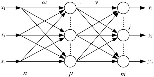
FIGURE 1. Back propagation neural network structure.

Here, n and m are the dimensions of the input layer and output layer data sets, corresponding to the number of independent variables and dependent variables in the actual research problem, p is the number of neurons in the hidden layer, and the number of neurons in each layer can also be called the number of nodes. ω_ij (i = 1, 2, … , n) and v_jk (j = 1, 2, … , p; k = 1, 2, … , m)are the connection weights between the layers, respectively. The steps of the classic BP algorithm are as follows:

Step 1. Forward calculation for unit j on the lth layer

where $y_j^{(l-1)}(n)$ is the signal transmitted by unit i of the previous layer (l-1). If the function of unit j is the Sigmoid function, then

and

If neuron j belongs to the first hidden layer (l = 1),then

If the neuron belongs to the output layer (l = L), then

and

Step 2. Reverse calculation δ. For output units

For Hidden Units

Step 3. Correct the weights.

In actual situations, the degree of weight change will become more and more intense as the value of η increases, resulting in oscillations. On the contrary, if the value of η is smaller, the corresponding learning process will become more convergent, and the learning speed will also slow down.

Step 4. n = n + 1, enter a new sample until the expected requirements are met.

Although the BP neural network is the most widely used algorithm in artificial neural network, there exist the following defects (Huang et al., 2020; Yang et al., 2019).

1. The problem of local minimization. The traditional BP neural network is a local search optimization method. The weights of the network are adjusted gradually along the direction of local improvement. This makes the algorithm trap into a local extremum, and the weights converge to the local minimum.

2. The convergence speed is slow. Since the BP neural network algorithm is essentially a gradient descent method, the objective function to be optimized is very complex, so the “sawtooth phenomenon” will appear, and when the neuron output is approaching 0 or 1, some flat areas appear, in which the weight error changes little, making the training process almost come to a halt. The traditional one-dimensional search method cannot be used in the BP neural network model to find the step length of each iteration, but the updated rule of the step length must be preassigned to the network.

3. The overfitting phenomenon of predictive ability. In general, the predictive ability increases with the improvement of training ability. But this trend is not fixed. When reaching the limit, with the improvement of training ability, the predictive ability will decrease instead, hence appearing the “overfitting” phenomenon. This phenomenon is attributed to the fact that the network has grasped too many sample details, and the learned model cannot reflect the laws contained in the samples any more.

4. Sample dependency problem. The approximation and generalization ability of the network model is strongly linked to the typicality of the learning samples, and there exist difficulties to select typical samples from the problems to form the training set.

2.2 Genetic Algorithm Prediction Model

The GA is a parallel random search optimization method put forward by Professor Holland in 1962 to simulate natural genetic mechanisms and biological evolution theory (Bodenhofer, 2003). It introduces the biological evolution principle of “natural selection and survival of the fittest” in nature into the coded tandem population formed by optimized parameters. Individuals are screened according to the selected fitness function and through selection, crossover, and mutation in heredity, such that individuals with good fitness value are retained, while those with poor fitness value are eliminated. The new population inherits the previous generation's information and also performs better than the previous generation. This cycle is repeated until the conditions are met.

GA optimizes the ownership and threshold of the BP neural network using GAs. Each individual in the population contains a network ownership value and threshold. The individual calculates the individual fitness value through the fitness function. The GA finds the corresponding individual of the optimal fitness value through selection, crossover, and mutation. The BP neural network prediction obtains the optimal individual through the GA to assign initial weights and thresholds to the network, and the network is trained to predict the output of the function. The formula of the mean square error fitness function is:

where N represents the number of data items in the training data set, and t_i and o_i are the expected target and training output, respectively.

3 Wind Power Prediction Model Based on Differential Evolution–Back Propagation

In order to overcome the BP local minimum problem caused by the initial random weight parameters of the network, this article introduces the DE algorithm, combined with the global search evolution algorithm and the local search gradient algorithm, to overcome the local minimum problem with high generalization and fast convergence speed.

3.1 The Optimization Characteristics of Differential Evolution Algorithm

The DE algorithm is an efficient global optimization algorithm which is a heuristic search algorithm based on population, and each individual in the population corresponds to a solution vector (Das and Suganthan, 2010).

The DE algorithm generates population individuals by using floating-point vectors for encoding (Fan, 2009). In the process of DE algorithm optimization, first, two individuals are selected from the parent individuals to generate a difference vector; second, another individual is selected to sum with the difference vector to generate the experimental individual; the parent individual and the corresponding experimental individual are cross-operated to generate new offspring individuals; finally, the selection is made between the parent individuals and the qualified individuals are saved for the next generation population (Chidambaram et al., 2017; Ramos and Susteras, 2006).

The standard DE algorithm consists of four steps: initialization, mutation, crossover, and selection. As shown in Figure 2, this article adopts the DE/rand/1/bin mechanism. The details of each step are as follows:

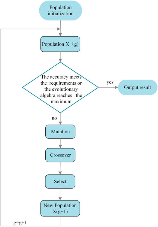
FIGURE 2. Flowchart of differential evolution algorithm.

Step 1. Initialization operation: The DE algorithm in this article adopts the real number coding method. In this step, the parameters are first initialized, including the population size N, gene dimension D, mutation factor F, crossover factor CR, and the value range of each gene [Umin, Umax], and then, the population is initialized randomly, as shown in the formula:

where i = 1, 2, … , N; j = 1, 2, … , D; rand is a random number that obeys a uniform distribution.

Step 2. Mutation operation: For each target vector $x_i^G,i=\mathrm{1,2},\dots ,N$, the standard DE algorithm generates a corresponding mutation vector by the formula:

Step 3.Crossover operation: Crossover operation generates an experimental individual by the formula:

where r(j) is a random number uniformly distributed among [0,1]; j represents the jth gene; the range of CR is [0,1]. In order to ensure the obtaining of at least one-dimensional variable of the experimental individual from the mutated individual, set rn(i) ∈ [1, 2, … , D] as a randomly selected gene dimension index. The smaller the CR, the better the global search effect.

Step 4. Selection operation: DE uses a greedy search strategy. Each target individual $x_i^G$ competes with its corresponding experimental individual $u_i^{G+1}$, and their fitness values are compared. Only when the fitness value of the experimental individual is better than that of the target individual can it be selected as the offspring. If not, the target individual is directly taken as the offspring. Taking minimization optimization as an example, the selection is demonstrated in Eq. 14, where f(.) is a fitness function:

As a new and efficient heuristic parallel search technology, the DE algorithm possesses such advantages as fast convergence, few control parameters, simple setting, and robust optimization results (Neri and Tirronen, 2010). It has important academic significance for the theory and application of evolutionary algorithms. However, the standard DE algorithm also has the phenomenon of high pressure of control parameter selection and the contradiction between search ability and development ability, which tends to cause such problems as premature convergence of individuals of the population and search stagnation.

3.2 Wind Power Prediction Method Based on Differential Evolution–Back Propagation Neural Network

Considering the shortcomings of the BP algorithm tending to fall into local optima, and the shortcomings of individual premature convergence and search stagnation of DE algorithm population, this article proposes a DE-BP algorithm for wind power prediction. First, the number of nodes of input, output, and hidden layer of the BP neural network are initialized, and traditional gradient descent and BP to adjust the weights and thresholds of the network to construct the BP neural network model are used. Secondly, the DE algorithm is introduced to optimize the initial connection weights and neuron thresholds of the BP neural network, which can avoid its falling into the local optimum. This article establishes a DE-BP neural network model based on the DE algorithm, which reduces the sensitivity of the BP neural network to the initial connection weights and neuron thresholds. The DE-BP model improves the speed and accuracy of network training. Since the BP algorithm is easy to fall into the local optimal value when predicting, the DE algorithm is introduced to optimize this shortcoming. The DE algorithm is used to optimize the initial weights and thresholds of the BP neural network, such that the optimized BP neural network can better predict samples. After the DE algorithm is optimized, the best initial weight and threshold matrix are obtained, and the initial weight and threshold are substituted into the network to obtain the training error value, predicted value, prediction error, and training error. The process of optimizing the BP neural network with the DE algorithm is shown in Figure 3.

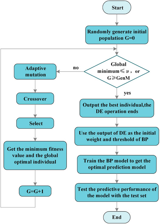
FIGURE 3. Flowchart of differential evolution–back propagation algorithm.

The initialization step of the DE algorithm first initializes the population size N, the individual gene dimension D, the maximum number of iterations G, the mutation factor F, the value range of each gene [Umin, Umax], and the crossover factor CR:

where i = 1, 2, … , N; j = 1, 2, … , D; rand is a random number that obeys the uniform distribution. It is determined whether the DE algorithm reaches the termination condition of the iteration. If it does, the DE process is stopped and the best individual is outputted; otherwise, the following operations are continued;

According to the adaptive mutation, crossover, and selection operation methods of the DE algorithm, the next generation of individuals $x_i^{G+1}$ is obtained; for each target vector $x_i^G,i=\mathrm{1,2},\dots ,N$, the DE algorithm generates a corresponding mutation:

where $x_{r_1}^G,x_{r_2}^G,x_{r_3}^G$ are the three individuals with different serial numbers. Among them, the individual serial numbers r₁, r₂, and r₃ are randomly selected, and they are different from each other and also different from the target individual's serial number i, so the population size N ≥ 4, among them:

where CR(g) represents the mutation probability of generation g; CR (g + 1), the mutation probability of generation g + 1; F_min is the smallest mutation factor; F_max is the largest mutation factor; GenM is the maximum number of iterations; G the current number of iterations; CR (0) is the initial value of the mutation factor; and CR_min is the minimum value of the mutation factor in the evolution process.

After the next generation of individuals is obtained, the fitness value of their population is evaluated. The minimum fitness value is the current global minimum value, and the corresponding individual is the current global optimal individual; then, let G = G + 1, returning to the judgment operation, the judgments are made based on the conditions. The optimal individual output optimized by the DE algorithm is used as the initial weight and threshold of BP, and the network is trained with a training set to obtain the optimal DE-BP prediction model. As shown in Figure 3, when the global minimum is ≤ μ or G ≥ GenM, the optimal individual is outputted and the DE operation ends. The termination condition in judging whether the DE algorithm reaches the termination condition of the iteration is: the minimum fitness value reaches the set error precision requirement μ or the algorithm has reached the maximum iteration number GenM.

4 Experiment Results

This article selects the historical data from a wind farm in Northwest China from October 2016 to April 2018, and samples wind speed, wind direction, temperature, and air pressure at the height of the turbine every 15 min. The 24-h wind power changes on 10 October 2016 are shown in Table1.

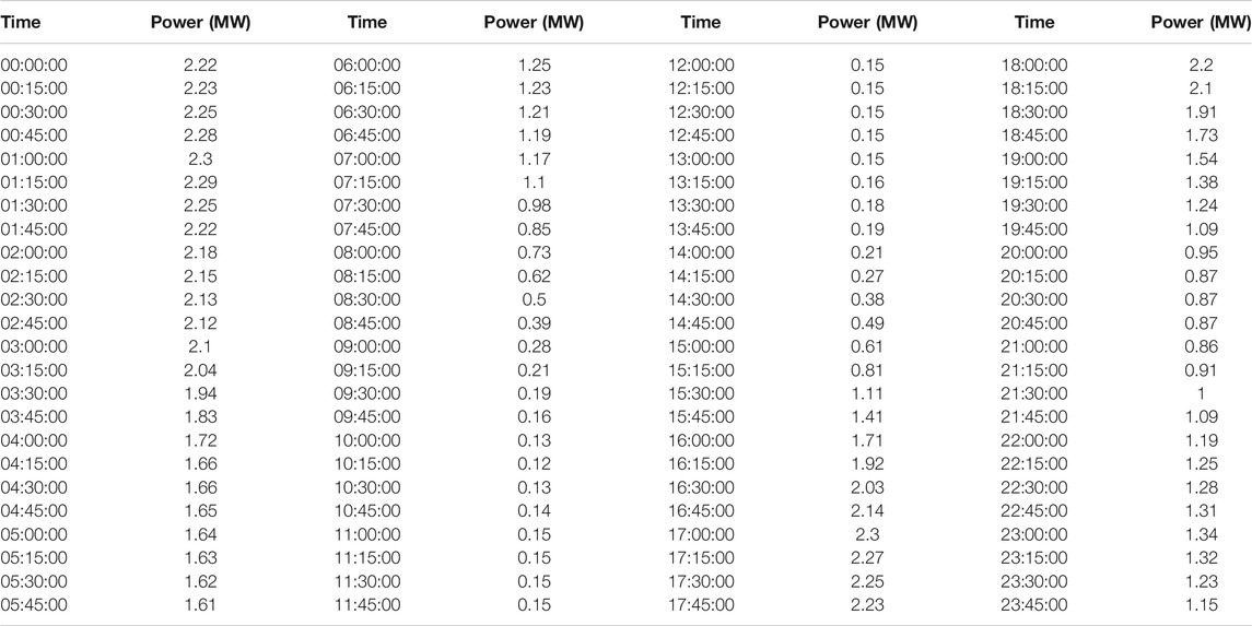
TABLE 1. Wind power changes on 10 October 2016.

A total of 5,000 samples and 4,000 sets of model parameter training samples were tested, and 1,000 samples were used as new data to verify the model. All algorithms were programmed by MATLAB, and 4,000 sets of data were randomly trained and 1,000 sets of data were tested. The corresponding wind speed fluctuations with time during wind power output are shown in Figure 4.

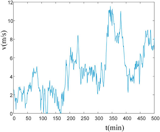
FIGURE 4. Wind speed distribution.

The error is shown in Table 2, when selecting a different mutation factor F and crossover factor CR for prediction. From Table 2, when F = 0.5 and CR = 0.6, the prediction error is the smallest, so this parameter is selected as the DE-BP prediction model parameter.

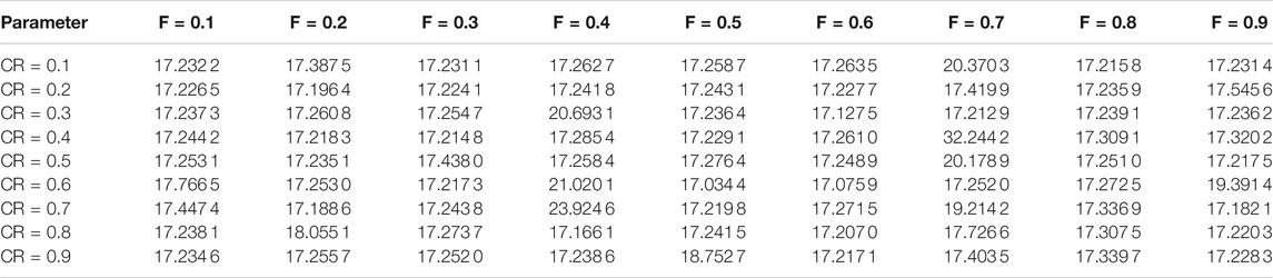
TABLE 2. Differential evolution–back propagation algorithm parameter selection.

The following three error assessment criteria analyze the feasibility and effectiveness of each model, that is, the mean absolute error (MAE), mean squared error (MSE), and root mean square error (RMSE). The formulas are as follows:

Table 3 lists the errors of using the BP neural network, GA-BP neural network, and DE-BP neural network to predict short-term wind power. The results show that, compared with other models, the DE-BP model has a higher prediction accuracy and stronger ability to track actual wind power. It can realize real-time wind power dispatching, reduce the damage to the wind power grid caused by random changes in wind power, and strengthen the emergency measures of dispatching organization for sudden wind power instability during the process of grid connection.

TABLE 3. Comparison of wind power prediction error results between back propagation (BP) and differential evolution (DE)–BP algorithms.

This article extracts 70 pieces of historical data as training samples and uses the trained network to predict the ultra-short-term wind power within 2 h after the prediction point. The prediction samples of each model are 30 prediction samples on a certain day. Taking into account the influence of the different climates and other factors throughout the year on wind power fluctuation, the wind power of each season is predicted, as shown in Figures 5A–D, representing spring, summer, autumn and winter, respectively.

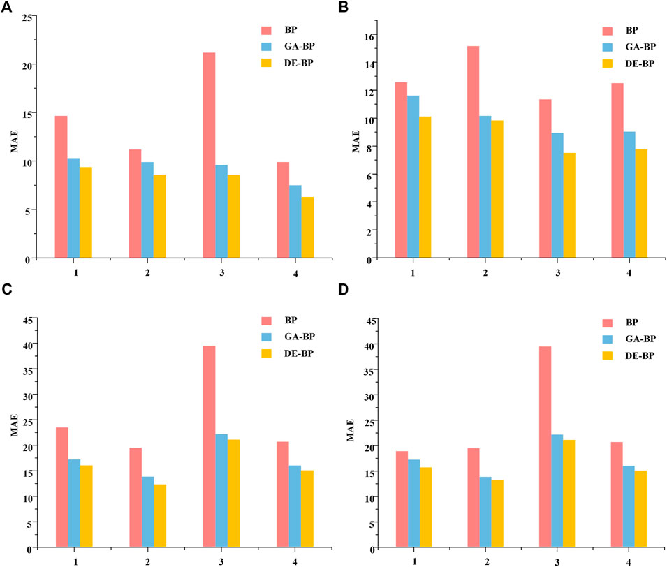
FIGURE 5. Comparison of prediction errors between differential evolution algorithm and other algorithms in each season: (A) spring, (B) summer, (C) fall, (D) winter.

Figure 6 shows the comparison of the prediction curves of short-term wind power prediction using each model. When the power fluctuation range is large, the DE-BP model has better tracking ability than the GA-BP and BP models. Combined with the error indicators in Table 4, the prediction error of the DE-BP model is relatively small.

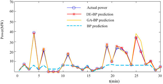
FIGURE 6. Comparison of the predicted value of differential evolution algorithm with other algorithms.

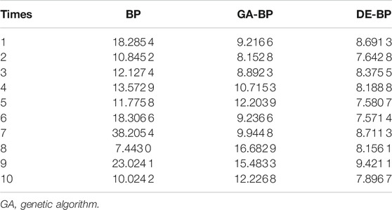
TABLE 4. Comparison of wind power prediction error results between back propagation (BP) and differential evolution (DE)–BP algorithms.

After the training of the BP neural network, the minimum fitness is found by the DE algorithm. The population size of the DE algorithm is 50, the number of iterations is 300, F = 0.5, and CR = 0.6, and the optimal individual fitness curve in the optimization process is shown in Figure 7. The optimal individual fitness value obtained by the DE-BP algorithm is less than 2.2 × 10^–3 and close to 0, indicating the effectiveness of the method.

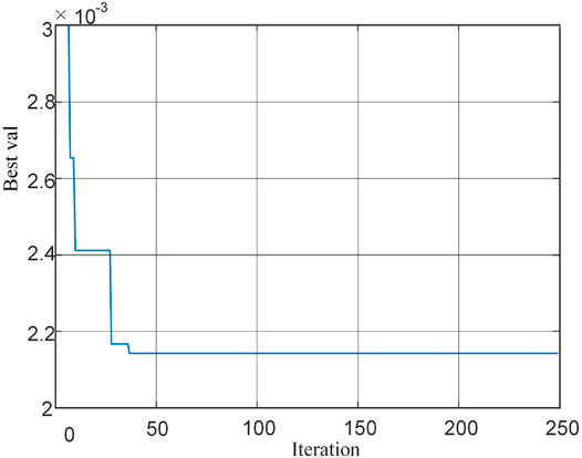
FIGURE 7. Differential evolution–back propagation algorithm fitness function changes.

The training time used by the two optimization models is shown in Table 5. The average training time of the GA-BP model is 86.245 3 s and that of the DE-BP model is 66.329 7 s. The parameters of the BP neural network can be optimized by the DE algorithm, which effectively improves the training time by 23.1%.

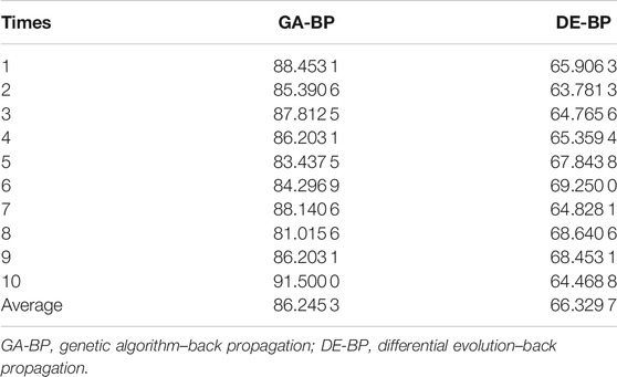
TABLE 5. Training time of wind power prediction model.

The corresponding errors of the three models in predicting short-term wind power are shown in Figure 8. It can be seen that the DE-BP wind power prediction model has the smallest error, which effectively improves the accuracy of the prediction.

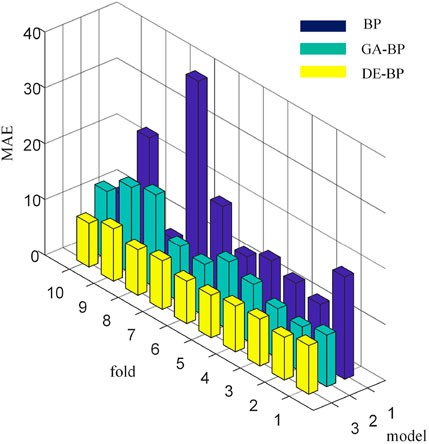
FIGURE 8. Error of wind power prediction model.

5 Conclusion

In recent years, as the proportion of wind power generation continues to increase, the research on the accuracy of wind power prediction has become extremely important. This article proposes a hybrid method for wind power prediction, which is based on a feedforward neural network trained through a combination of the DE and BP algorithms.

This article mainly studies the objective function and parameter optimization. The DE algorithm is used to optimize the weight threshold of the BP neural network, and its average MSE is used as the objective function to improve the stability and generalization performance of the model, and the prediction accuracy is more than 95%. The average MAE during model testing was 7.48, highlighting the effectiveness of the proposed method. Compared with the traditional BP and GA-BP algorithms, the accuracy is improved. Finally, the above optimization algorithm is applied to wind power prediction to improve the prediction accuracy and stability, improve the wind power absorption capacity, and provide a reference for power grid dispatching. By preprocessing the historical data of a wind farm in Northwest China, the classic BP prediction, GA-BP prediction, and DE-BP prediction models are established and compared through simulation. It is verified that the DE-BP model is superior to the other models in terms of prediction, fills the gap of DE-BP in the field of wind power prediction, and has good prospect of engineering research value.

Data Availability Statement

The raw data supporting the conclusion of this article will be made available by the authors, without undue reservation.

Author Contributions

NL is the corresponding author and takes primary responsibility. YW contributed for analysis of the work and wrote the first draft of the manuscript. All authors contributed to manuscript revision, and read and approved the submitted version.

Funding

This work was supported in part by the National Natural Science Foundation of China (52177193); China Scholarship Council (CSC) State Scholarship Fund International Clean Energy Talent Project (Grant No (2018)5046,(2019)157); and Open Research Fund of Jiangsu Collaborative Innovation Center for Smart Distribution Network, Nanjing Institute of Technology (XTCX202107).

Conflict of Interest

The authors declare that the research was conducted in the absence of any commercial or financial relationships that could be construed as a potential conflict of interest.

Publisher’s Note

All claims expressed in this article are solely those of the authors and do not necessarily represent those of their affiliated organizations, or those of the publisher, the editors, and the reviewers. Any product that may be evaluated in this article, or claim that may be made by its manufacturer, is not guaranteed or endorsed by the publisher.

References

Agarwal, P., Shukla, P., and Sahay, K. B. (2018). “A Review on Different Methods of Wind Power Forecasting,” in Proceeding of the 2018 International Electrical Engineering Congress (iEECON), Krabi, Thailand, 7-9 March 2018 (IEEE), 1–4. doi:10.1109/IEECON.2018.8712262
Babazadeh, H., Gao, W., Cheng, L., and Lin, J. (2012). “An Hour Ahead Wind Speed Prediction by Kalman Filter,” in Proceeding of the 2012 IEEE Power Electronics and Machines in Wind Applications, Denver, CO, USA, 16-18 July 2012 (IEEE), 1–6.
Bhaskar, K., and Singh, S. N. (2012). Awnn-assisted Wind Power Forecasting Using Feed-Forward Neural Network. IEEE Trans. Sustain. Energ. 3, 306–315. doi:10.1109/tste.2011.2182215
Bodenhofer, U. (2003). “Genetic Algorithms: Theory and Applications,” in Lecture Notes, Fuzzy Logic Laboratorium Linz-Hagenberg, Winter 2004.
Catalao, J. P. S., Pousinho, H. M. I., and Mendes, V. M. F. (2009). “An Artificial Neural Network Approach for Short-Term Wind Power Forecasting in portugal,” in Proceeding of the 2009 15th International Conference on Intelligent System Applications to Power Systems, Curitiba, Brazil, 8-12 Nov. 2009 (IEEE), 1–5. doi:10.1109/ISAP.2009.5352853
Chandra, D. R., Kumari, M. S., and Sydulu, M. (2013). “A Detailed Literature Review on Wind Forecasting,” in Proceeding of the 2013 International Conference on Power, Energy and Control (ICPEC), Dindigul, India, 6-8 Feb. 2013 (IEEE), 630–634.doi:10.1109/ICPEC.2013.6527734
Chang, W.-Y. (2014). A Literature Review of Wind Forecasting Methods. Jpee 02, 161–168. doi:10.4236/jpee.2014.24023
Chidambaram, B., Ravichandran, M., Seshadri, A., and Muniyandi, V. (2017). Computational Heat Transfer Analysis and Genetic Algorithm–Artificial Neural Network–Genetic Algorithm-Based Multiobjective Optimization of Rectangular Perforated Plate Fins. IEEE Trans. Components, Packaging Manufacturing Technology 7, 208–216. doi:10.1109/TCPMT.2016.2646718
Das, S., and Suganthan, P. N. (2010). Differential Evolution: A Survey of the State-Of-The-Art. IEEE Trans. Evol. Comput. 15, 4–31. doi:10.1109/TEVC.2010.2059031
Foley, A. M., Leahy, P. G., Marvuglia, A., and McKeogh, E. J. (2012). Current Methods and Advances in Forecasting of Wind Power Generation. Renew. Energ. 37, 1–8. doi:10.1016/j.renene.2011.05.033
Haque, A. U., Mandal, P., Meng, J., Srivastava, A. K., Tseng, T.-L., and Senjyu, T. (2013). A Novel Hybrid Approach Based on Wavelet Transform and Fuzzy Artmap Networks for Predicting Wind Farm Power Production. IEEE Trans. Ind. Applicat. 49, 2253–2261. doi:10.1109/tia.2013.2262452
Hongmei Fan, H. (2009). Using Radiating Near Field Region to Sample Radiation of Microstrip Traces for Far Field Prediction by Genetic Algorithms. IEEE Microw. Wireless Compon. Lett. 19, 272–274. doi:10.1109/lmwc.2009.2017586
Huang, Y., Xiang, Y., Zhao, R., and Cheng, Z. (2020). Air Quality Prediction Using Improved Pso-Bp Neural Network. Ieee Access 8, 99346–99353. doi:10.1109/access.2020.2998145
Ju, Y., Sun, G., Chen, Q., Zhang, M., Zhu, H., and Rehman, M. U. (2019). A Model Combining Convolutional Neural Network and Lightgbm Algorithm for Ultra-short-term Wind Power Forecasting. Ieee Access 7, 28309–28318. doi:10.1109/access.2019.2901920
Li, N., He, F., Ma, W., Wang, R., and Zhang, X. (2020). Wind Power Prediction of Kernel Extreme Learning Machine Based on Differential Evolution Algorithm and Cross Validation Algorithm. IEEE Access 8, 68874–68882. doi:10.1109/access.2020.2985381
Liu, L. (2019). Recognition and Analysis of Motor Imagery Eeg Signal Based on Improved Bp Neural Network. IEEE Access 7, 47794–47803. doi:10.1109/access.2019.2910191
Liu, Y., Sun, Y., Infield, D., Zhao, Y., Han, S., and Yan, J. (2016). A Hybrid Forecasting Method for Wind Power Ramp Based on Orthogonal Test and Support Vector Machine (Ot-svm). IEEE Trans. Sustainable Energ. 8, 451–457. doi:10.1063/1.4950972
Liu, Z., Tan, Q., Zhou, Y., and Xu, H. (2021). Syncretic Application of Ibas-Bp Algorithm for Monitoring Equipment Online in Power System. IEEE Access 9, 21769–21776. doi:10.1109/access.2021.3055247
Neri, F., and Tirronen, V. (2010). Recent Advances in Differential Evolution: a Survey and Experimental Analysis. Artif. Intell. Rev. 33, 61–106. doi:10.1007/s10462-009-9137-2
Paula, M., Marilaine, C., Jose Nuno, F., and Wallace, C. (2020). Predicting Long-Term Wind Speed in Wind Farms of Northeast brazil: A Comparative Analysis through Machine Learning Models. IEEE Latin Am. Trans. 18, 2011–2018. doi:10.1109/tla.2020.9398643
Ramos, D. S., and Susteras, G. L. (2006). Applying Genetic Algorithms for Predicting Distribution Companies Power Contracting. IEEE Latin Am. Trans. 4, 268–278. doi:10.1109/tla.2006.4472123
Shen, T., Chang, J., and Liang, Z. (2020). Swarm Optimization Improved Bp Algorithm for Microchannel Resistance Factor. IEEE Access 8, 52749–52758. doi:10.1109/access.2020.2969526
Sideratos, G., and Hatziargyriou, N. D. (2007). An Advanced Statistical Method for Wind Power Forecasting. IEEE Trans. Power Syst. 22, 258–265. doi:10.1109/TPWRS.2006.889078
Tan, L., Han, J., and Zhang, H. (2020). Ultra-short-term Wind Power Prediction by Salp Swarm Algorithm-Based Optimizing Extreme Learning Machine. IEEE Access 8, 44470–44484. doi:10.1109/access.2020.2978098
Tasnim, S., Rahman, A., Shafiullah, G., Oo, A. M. T., and Stojcevski, A. (2014). “A Time Series Ensemble Method to Predict Wind Power,” in Proceeding of the 2014 IEEE symposium on computational intelligence applications in smart grid (CIASG), Orlando, FL, USA, 9-12 Dec. 2014 (IEEE), 1–5. doi:10.1109/CIASG.2014.7011544
Wan, C., Xu, Z., Pinson, P., Dong, Z. Y., and Wong, K. P. (2014). Probabilistic Forecasting of Wind Power Generation Using Extreme Learning Machine. IEEE Trans. Power Syst. 29, 1033–1044. doi:10.1109/TPWRS.2013.2287871
Wu, W., Feng, G., Li, Z., and Xu, Y. (2005). Deterministic Convergence of an Online Gradient Method for Bp Neural Networks. IEEE Trans. Neural Netw. 16, 533–540. doi:10.1109/tnn.2005.844903
Wu, Y.-K., Su, P.-E., and Hong, J.-S. (2016). “An Overview of Wind Power Probabilistic Forecasts,” in Proceeding of the 2016 IEEE PES Asia-Pacific Power and Energy Engineering Conference (APPEEC), Xi'an, China, 25-28 Oct. 2016 (IEEE), 429–433. doi:10.1109/APPEEC.2016.7779540
Xiong, L., Liu, X., Liu, Y., and Zhuo, F. (2020). Modeling and Stability Issues of Voltage-Source Converter Dominated Power Systems: A Review. CSEE J. Power Energ. Syst. doi:10.17775/CSEEJPES.2020.03590
Yan, J., Zhang, H., Liu, Y., Han, S., Li, L., and Lu, Z. (2017). Forecasting the High Penetration of Wind Power on Multiple Scales Using Multi-To-Multi Mapping. IEEE Trans. Power Syst. 33, 3276–3284. doi:10.1109/TPWRS.2017.2787667
Yang, A., Zhuansun, Y., Liu, C., Li, J., and Zhang, C. (2019). Design of Intrusion Detection System for Internet of Things Based on Improved Bp Neural Network. IEEE Access 7, 106043–106052. doi:10.1109/access.2019.2929919
Yuqin, X., Yang, N., and Wenxia, L. (2014). “Predicting Available Transfer Capability for Power System with Large Wind Farms Based on Multivariable Linear Regression Models,” in Proceeding of the 2014 IEEE PES Asia-Pacific Power and Energy Engineering Conference (APPEEC), Hong Kong, China, 7-10 Dec. 2014 (IEEE), 1–6. doi:10.1109/APPEEC.2014.7066008
Zhang, H., Liu, Y., Yan, J., Han, S., Li, L., and Long, Q. (2020). Improved Deep Mixture Density Network for Regional Wind Power Probabilistic Forecasting. IEEE Trans. Power Syst. 35, 2549–2560. doi:10.1109/tpwrs.2020.2971607
Zhang, Y., Sun, H., and Guo, Y. (2019). Wind Power Prediction Based on Pso-Svr and Grey Combination Model. IEEE Access 7, 136254–136267. doi:10.1109/access.2019.2942012
Keywords: differential evolution algorithm, wind power prediction, BP neural network, prediction time, accuracy
Citation: Li N, Wang Y, Ma W, Xiao Z and An Z (2022) A Wind Power Prediction Method Based on DE-BP Neural Network. Front. Energy Res. 10:844111. doi: 10.3389/fenrg.2022.844111
Received: 27 December 2021; Accepted: 18 January 2022;
Published: 15 February 2022.
Edited by:
Liansong Xiong, Nanjing Institute of Technology (NJIT), ChinaReviewed by:
He Li, Xidian University, ChinaYingjie Wang, University of Liverpool, United Kingdom
Jianquan Shi, Nanjing Institute of Technology (NJIT), China
Copyright © 2022 Li, Wang, Ma, Xiao and An. This is an open-access article distributed under the terms of the Creative Commons Attribution License (CC BY). The use, distribution or reproduction in other forums is permitted, provided the original author(s) and the copyright owner(s) are credited and that the original publication in this journal is cited, in accordance with accepted academic practice. No use, distribution or reproduction is permitted which does not comply with these terms.
*Correspondence: Ning Li, lining83@xaut.edu.cn