Development and Assessment of an Isotropic Four-Equation Model for Heat Transfer of Low Prandtl Number Fluids

1 Introduction

Liquid metals are widely considered coolants with good thermal-hydraulic characteristics for many energy systems, such as fast reactors and subcritical reactors (Gu and su, 2021; Wang et al., 2021). However, liquid metals’ low molecular Prandtl number $Pr$ leads to special heat transfer compared to traditional fluids. Typically, the $Pr$ of lead-bismuth is 0.03–0.01 and that of sodium is 0.01–0.006 (Vià et al., 2020). It is significant to study liquid metals’ turbulent heat transfer characteristics, which will affect the economy and security of the energy system.

It is difficult, dangerous, and costly to experiment with liquid metals (Schroer et al., 2012; Ejenstam and Szakálos, 2015), while the computational fluid dynamics (CFD) method is more commonly applied to investigate the thermal-hydraulic properties of these liquids. However, in CFD, the computing cost required by the direct numerical simulation (DNS) method and the large eddy simulations (LES) method is too high to rely on this technique for a quick and economic calculation of heat transfer in complex geometries (Kawamura et al., 1999), while the Reynolds Averaged Navier–Stokes (RANS) method can be promoted. The velocity boundary layer and the temperature layer of traditional fluid (Pr ≈ 1) are generally considered to be similar in the RANS framework. In this way, one can obtain a constant turbulent Prandtl number $P{r}_t$ to simplify the calculation of the energy equation after using the simple gradient diffusion hypothesis (SGDH) (Groetzbach, 2013). However, it is invalid for low Pr fluids (Reynolds, 1975).

In the SGDH framework, Cheng (Cheng and Tak, 2006) derived a $P{r}_t$ correlation through employing global Reynolds numbers, while Kays (Kays, 1994) introduced the local turbulence effect into the $P{r}_t$ relation. These nonlinear $P{r}_t$ relations can effectively improve this problem in some simple geometries. However, these relations still need to be further verified in complex geometries (Duponcheel et al., 2014). Unlike the SGDH method, the differential or algebraic heat flux model (D/AHFM) establishes differential or algebraic transport equations to consider the dissimilarity between velocity and the temperature field to improve the heat transfer accuracy of liquid metals. Assessment and calibration results of D/AHFM models for low $Pr$ fluids completed in some simple geometries show that the heat transport of second-moment closure is very sensitive to the model coefficients and functions (Lai and So, 1990; Shikazono and Kasagi, 1996; Choi and Kim, 2007; Shams et al., 2019).

Another popular model in the SGDH work, called the four-equation k-ε-k_θ-ε_θ turbulent heat transfer model, is introduced into turbulent and thermal time-scales for the simulation of the explicit first-order turbulent heat diffusivity. The literature (Nagano and Kim, 1988; Abe et al., 1995; Nagano and Shimada. 1996) has contributed extensively to near-wall model closure and thermal turbulence effect for a four-equation model. In recent years, Manservisi (Manservisi and Menghini, 2014a) improved the four-equation k-ε-k_θ-ε_θ model proposed by Abe and Nagano. The model predicted the heat transfer process of the plane, circular tube, triangular rod bundles, and quadrilateral rod bundles for $Pr=0.025$ fluids (Manservisi and Menghini, 2014b; Manservisi and Menghini, 2015). However, the numerical stability of the four-equation model is affected by its near-wall boundary conditions. To improve the problem, a four-equation k-ω-k_θ-ω_θ model with the specific dissipation rates ω = ε/(C_μk) and ω_θ = ε_θ/(C_μk_θ) was developed based on Manservisi’s k-ε-k_θ-ε_θ model (Cerroni et al., 2015). Then by the following work of the literatures (Vià et al., 2016; Chierici et al., 2019; Vià and Manservivi, 2019), logarithmic specific dissipation rates of ω and ω_θ, that is, Ω = ln(ω) and Ω_θ = ln (ω_θ), have been used to simplify the near-wall boundary conditions and have been introduced into the logarithmic four-equation k-Ω-k_θ-Ω_θ model. Other state variables as proposed by Youssef (Youssef, 2006) are the velocity τ_u = k/ε and temperature time-scale τ_θ= k_θ/ε_θ to improve its numerical stability. The proposed k_θ-τ_θ model does not suffer from numerical stiffness problems since natural boundary conditions for the variables k_θ and τ_θ are used (k_θ = τ_θ = 0, at walls). In addition, the static variables $\tilde{\epsilon }$ and $\widetilde{{\epsilon }_{\theta }}$, called the isotropic dissipation rates, which are linked to the “true” dissipation rates ε and ε_θ, can also provide Dirichlet wall boundary conditions and simpler transport modes than the k_θ-τ_θ modes (Nagano and Shimada, 1996; Nagano et al., 1997).

However, the application codes of an isotropic four-equation model in complex geometries are still lacking for liquid metals, and its reliability needs to be further verified and evaluated. So, in the present work, the four-equation model in an isotropic dissipation rate $k-\tilde{\epsilon }-k_{\theta }-\widetilde{{\epsilon }_{\theta }}$ formulation for liquid metals to improve its numerical robustness was presented by Taylor series expansion and near-wall turbulence analysis based on Abe’s model and Manservisi’s model. The turbulent heat transfer process of $Pr$ = 0.01 ∼ 0.05 fluids in parallel planes is numerically studied based on the finite volume method and the open-source CFD program OpenFOAM. The validity of the present four-equation model was verified by DNS data. To evaluate the present model’s applicability in complex geometries, the turbulent heat transfer of $Pr=0.01$ fluids in a bare quadrilateral infinite rod bundle with different pitch-to-diameter ratios is predicted on the present isotropic four-equation model. The numerical results obtained from two SGDH options, the $P{r}_t=0.85$ model and the present isotropic $k-\tilde{\epsilon }-k_{\theta }-\widetilde{{\epsilon }_{\theta }}$ model, are compared and analyzed with the available experimental relations and CFD results. The local distributions of dimensionless temperature, temperature fluctuation, turbulent heat diffusivity, and turbulent Prandtl numbers are analyzed.

2 Mathematical Model

2.1 Isotropic Four-Equation Turbulence Model

The incompressible RANS equations with no gravity and constant physical properties for the calculation of velocity, pressure, and temperature fields are considered as follows:

where $u_i$, $P$, and $T$ are the RANS velocities, pressure, and temperature fields. $\nu$, $\rho$, and $\alpha$ are the molecular viscosity, density, and molecular thermal diffusivity, respectively. The Reynolds stress $\overline{u_i^{\prime }{u}_j^{\prime }}$ using the Boussinesq hypothesis and Reynolds flux $\overline{u_j^{\prime }{T}^{\prime }}$ using the SGDH are set as follows:

The turbulent viscosity ${\nu }_t$ can be solved using two-equation $k-\epsilon$ or $k-\omega$ models, while the turbulent thermal diffusivity ${\alpha }_t$ is considered as follows:

Due to low Pr fluids’ physical properties, there are great differences between the momentum and heat. A constant Pr_t ≈ 0.85–0.9 cannot give acceptable results for liquid metals. It is possible to consider ${\alpha }_t$ as a function of the turbulence variables, such as two-equation $k_{\theta }-{\epsilon }_{\theta }$ or $k_{\theta }-{\omega }_{\theta }$ analogy to dynamic two-equation $k-\epsilon$ or $k-\omega$. To smooth the isotropic variables at the wall, when one makes $\tilde{\epsilon }$ and $\widetilde{{\epsilon }_{\theta }}$ zero at the wall, an isotropic four-equation $k-\tilde{\epsilon }-k_{\theta }-\widetilde{{\epsilon }_{\theta }}$ model can be written using the Taylor series expansion as follows:

where $\tilde{\epsilon }$ and $\widetilde{{\epsilon }_{\theta }}$ call the isotropic dissipation rate. $\epsilon$ and ${\epsilon }_{\theta }$ are the “true” dissipation rate, respectively. $f_{\epsilon }$, $f_w$, $f_{d2}$, and $f_{w\theta }$ are wall-proximity effect functions. Based on the analysis of the literature and the DNS database (Abe et al., 1995; Kawamura et al., 1998; Manservisi and Menghini, 2014a), the isotropic four-equation model coefficients for liquid metals are used and corrected as shown in Table 1. Here, the $k-\tilde{\epsilon }-k_{\theta }-\widetilde{{\epsilon }_{\theta }}$ model functions and constants recommended in this study, such as $f_{\epsilon }$, $f_w$, $f_{d2}$, $f_{w\theta }$, and $C_{d1}$, are different from the $k-\epsilon -k_{\theta }-{\epsilon }_{\theta }$ model values of Manservisi (Manservisi and Menghini, 2014b). It is noted that $P_{k\theta }$ is the production term of temperature fluctuations $k_{\theta }$, which represents the energy transferred to the turbulent flux by the average temperature change rate of the RANS flow. That is, the temperature fluctuations $k_{\theta }$ is the result of the combined action of the average temperature change rate and Reynolds heat flux. Through the transport of Eq. 11, after the temperature fluctuation occurs, it will experience convection, molecular diffusion, and turbulent diffusion until it is dissipated.

TABLE 1. Values for the $k-\tilde{\epsilon }-k_{\theta }-\widetilde{{\epsilon }_{\theta }}$ model constants in Eqs 9–12.

Both the turbulent Reynolds number $R_t=k^2/\nu \epsilon$ and $R_{\epsilon }$ are introduced into the isotropic model. Let $\delta$ be the wall distance. $R_{\epsilon }$ can be recommended by Abe et al. (Abe et al., 1995), as follows:

where $\eta ={\left({\nu }^3/\epsilon \right)}^{1/4}$ is the Kolmogorov length scale which can calculate the separated flow well. When isotropic variables are used, $R_t$ and $R_{\epsilon }$ in Eqs 14–17 should become the following:

2.2 Turbulent Viscosity and Turbulent Thermal Diffusivity

Some dynamic and thermal time-scales should be applied to calculate the turbulent viscosity ${\nu }_t$ and turbulent thermal diffusivity ${\alpha }_t$. Using dynamic and thermal time-scales, that is, ${\tau }_u=k/\epsilon$ and ${\tau }_{\theta }=k_{\theta }/{\epsilon }_{\theta }$, turbulent viscosity and turbulent thermal diffusivity can be defined (Abe et al., 1995; Manservisi and Menghini, 2015) as follows:

where

and

where

and

The above model has been proved to be effective in producing correct turbulence behavior of liquid metal, which draws into the mixing time-scale ${\tau }_m={\tau }_{u}R/\left(C_m+R\right)$ and the ratio of the velocity time-scale to the thermal time-scale $R={\tau }_{\theta }/{\tau }_u$ (Abe et al., 1995). The values of $P{r}_{t\infty }=0.9$ and $C_m=0.3$ are recommended for liquid metals (Manservisi and Menghini, 2015). In order to establish a complete isotropic four-equation turbulent heat transfer model $k-\tilde{\epsilon }-k_{\theta }-\widetilde{{\epsilon }_{\theta }}$, we used the isotropic variables $\tilde{\epsilon }$ and $\widetilde{{\epsilon }_{\theta }}$ in Eqs 20–26 instead of the “true” variables $\epsilon$ and ${\epsilon }_{\theta }$.

2.3 Wall Boundary Conditions for Turbulence Models

Appropriate boundary conditions should be applied to solve the four-equation turbulent models without the available wall functions. By using series expansions as shown in Table 2, the near-wall behaviors of dynamical and thermal turbulence variables $k, \epsilon , k_{\theta }$, and ${\epsilon }_{\theta }$ can be obtained (Deng et al., 2001) as follows:

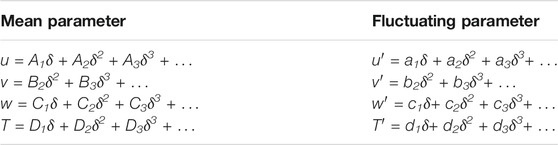
TABLE 2. Series expansion near the wall.

According to the definitions of Eqs 7, 8, when $\delta$ tends to zero, $k$, $\tilde{\epsilon }$, $k_{\theta }$, and $\widetilde{{\epsilon }_{\theta }}$ tend to zero. Thus, the simple Dirichlet wall boundary conditions with the isotropic $k-\tilde{\epsilon }-k_{\theta }-\widetilde{{\epsilon }_{\theta }}$ model can be imposed.

2.4 Modified Navier–Stokes Equations for Periodic Boundary Conditions

For a fully developed turbulent field, the pressure gradient term in Eq. 2 is divided into the mean of the pressure gradient $d{P}_f/dz$ which is constant along the flow direction $z$ and the fluctuating pressure gradient $\partial P/\partial x_i$. The mean term of the pressure gradient is given as the known power source term.

For a fully developed temperature field, temperature T is written as follows:

where $T_{in}$ is the inlet temperature, and $\Delta T_b$ is a constant wall temperature gradient, while $\theta$ satisfies periodic boundary conditions along the flow direction. According to the energy conservation for thermal fully developed flow with a wall flux $q_w$, $\Delta T_b$ can be set as $4q_w/\left(\rho C_p{u}_b{D}_h\right)$, where $u_b$ is average velocity, and $D_h$ is an equivalent diameter. After introducing periodic temperature $\theta$, Eq. 3 can be written as follows:

3 Numerical Results and Analysis

3.1 Numerical Solver of the Isotropic Four-Equation Model

For the modified RANS system and the isotropic four-equation $k-\tilde{\epsilon }-k_{\theta }-\widetilde{{\epsilon }_{\theta }}$ model in Section 2, the appropriate discrete format could be selected according to the needs. Here, the convection term adopts the Gauss upwind format, the diffusion term uses the Gauss linear format, and the time term uses the steady-state format. The SIMPLE algorithm solves the continuity and momentum simultaneously, and coupled multigrid iteration is used for the matrix solution. The convergence conditions of residual error are as follows:

where Q stands for $u_i,\theta , k, \tilde{\epsilon }, k_{\theta } \text{and }\widetilde{{\epsilon }_{\theta }}$. The index $i$ denotes the steps of calculation. All calculations were realized on OpenFOAM (Weller et al., 1998; Moukalled et al., 2016). The detailed analysis of the four-equation model solver by Gu and Su (Gu and su, 2021) based on OpenFOAM can be further referred to. The height of the grid point closest to the wall is approximately ${10}^{-3}$ mm to meet the requirements of the isotropic four-equation model ($y^{+}<1$).

3.2 Numerical Verification of the Plane

The full development process of different Pr fluids in a constant heat flow heated plane was studied using DNS (Kawamura et al., 1998; Kawamura et al., 1999; Tiselj and Cizelj, 2012). This study compares the DNS data with Pr = 0.01 ∼ 0.05. The plane geometry and mesh parameters are consistent with those in the literature (Su et al., 2021; Su and Gu, 2021). Here, the three-dimensional parallel plane with a flow length of 6.4 h, a spanwise width of 3.2 h, and a plane height of 2 h were selected as the calculation domain, where h is the half-height of the plane, 30.25 mm. The wall heat flux is set as q_w = 360 kW/m². Finally, 80, 50, and 100 nodes are divided into three directions, respectively: Flow direction, span direction, and height. Due to the symmetry of the plane, half of the plane is taken as the calculation domain, and the structured grid is used. The grid height of the first boundary layer is set to 3 × 10⁻⁶ m to meet the requirements of the low Reynolds number turbulence model, $y^{+}<1$. The physical properties of $Pr$ = 0.01–0.05 are reported in Table 3. The friction Reynolds number $R{e}_{\tau }=u_{\tau }h/\nu$ is taken as the calculation conditions: 180 (A), 395 (B), 590 (C), 640 (D), 950 (E), 2000 (F), and 4,400 (G), where $u_{\tau }$ is the friction velocity on the wall side, $h$ is the half-height of the plane, and the numbers A ∼ G represent different Reynolds number calculation conditions. For the convenience of analysis, $u_{\tau }$ and the friction temperature $T_{\tau }$ are taken as the dimensionless reference quantity, where $T_{\tau }$ is set as $q_w{\rho }^{-1}C{p}^{-1}{u}_{\tau }^{-1}$, and $q_w$ is the wall heat flux.

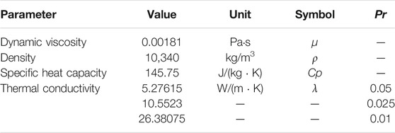
TABLE 3. Physical properties for Pr = 0.01, 0.025, and 0.05

3.2.1 Velocity Field Verification

The dimensionless velocity $u^{+}=u/u_{\tau }$ distribution of cases A and F along the dimensionless wall-normal distance $y^{+}=y{u}_{\tau }/v$ is shown in Figure 1. At a low Reynolds number and a high Reynolds number, the velocity distribution predicted by the present isotropic four-equation model is in good agreement with the DNS results, and the velocity distribution meets u⁺ = y⁺ in the linear region (u⁺ = y⁺) while it meets u⁺ = 2.5ln y⁺+5 in the logarithmic rate region (y⁺ > 30).

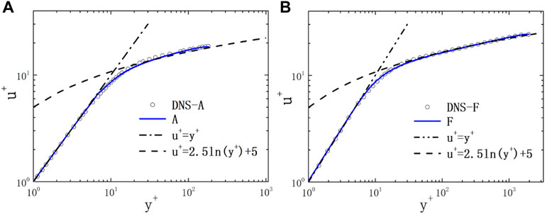
FIGURE 1. Non-dimensional velocity of the plane. (A) case A; (B) case F.

The distribution of dimensionless Reynolds stress ${\tau }_R^{+}=\overline{u\upsilon }{u}_{\tau }^{-2}$ and total shear stress ${\tau }_{total}^{+}={\tau }_R^{+}+\nu {\upsilon }_{,y}{u}_{\tau }^{-2}$ along $y^{+}$ under cases A and F is shown in Figure 2. The stress calculation results are in good agreement with DNS results. In the near-wall region (1 < y⁺ < 7), this study predicted ${\tau }_R^{+}$ to be lower than the DNS value. However, it has little effect on the calculation results of the velocity field in the linear region, mainly because the molecular diffusion is dominant in the near-wall region. With the increase in wall distance, the turbulent diffusion effect increases gradually. When y⁺ > 30, the total shear stress coincides with the Reynolds stress curve.

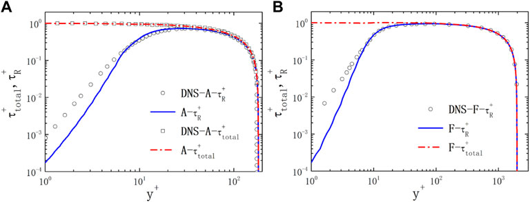
FIGURE 2. Non-dimensional stress of the plane. (A) case A; (B) case F.

3.2.2 Temperature Field Verification

1) Pr = 0.01

The dimensionless temperature ${\theta }^{+}=\theta /T_{\tau }$ distribution of the Pr = 0.01 fluid along $y^{+}$ is shown in Figure 3A. Cases A, B, and C agree with DNS and meet θ⁺ = Pry⁺ in the linear region (1 < y⁺ < 40).

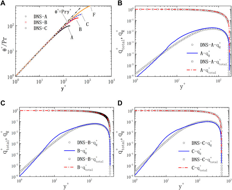
FIGURE 3. Non-dimensional temperature and heat flux of the plane for Pr = 0.01. (A) temperature; (B) heat flux of case A; (C) heat flux of case B; (D) heat flux of case C.

The distribution of dimensionless Reynolds heat flux $q_R^{+}=-{\alpha }_t{\theta }_{,y}{u}_{\tau }^{-1}{T}_{\tau }^{-1}$ and total heat flux $q_{total}^{+}=-\left({\alpha }_t+\alpha \right){\theta }_{,y}{u}_{\tau }^{-1}{T}_{\tau }^{-1}$ along $y^{+}$ is shown in Figures 3B–D. The heat flux calculation results of cases A–C are in good agreement with DNS results. Due to the thick thermal boundary layer and strong molecular heat conduction of low Pr fluid, although the predicted Reynolds heat flux deviates from the DNS results at 1 < y⁺ < 30, it does not affect the linear distribution of the temperature field in this region. With the increase in wall distance, although the effect of turbulent heat diffusion is gradually increasing, there is still a difference between the total heat flow and Reynolds heat flux, mainly caused by the strong molecular heat conduction of low Pr fluid.

2) Pr = 0.025

The distribution of θ⁺/Pr of the $Pr=0.025$ fluid along $y^{+}$ is shown in Figure 4A. Cases A, B, and C are in good agreement with DNS. The peak value of θ⁺/Pr increases with the increase in the Reynolds number. The distribution of $q_R^{+}$ along $y^{+}$ is shown in Figure 4B. Cases A and B agree with DNS. With the increase in Re, the $q_R^{+}$ peak increases and moves to the turbulent core.

3) Pr=0.05

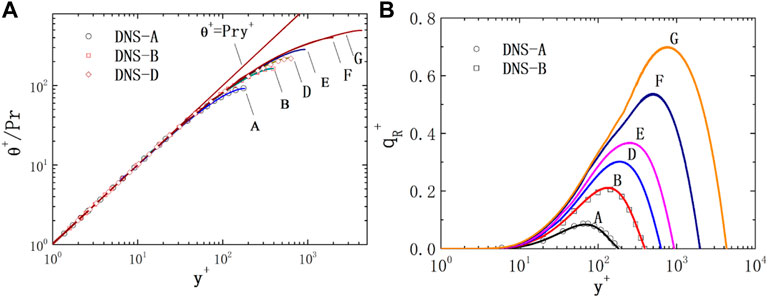
FIGURE 4. Non-dimensional temperature and heat flux of the plane for Pr = 0.025. (A) temperature; (B) heat flux.

As shown in Figure 5A, the dimensionless temperature θ⁺ of case A of Pr = 0.05 fluid is in good agreement with the DNS results. At the same Reynolds number, with the decrease in Pr, the molecular thermal conductivity increases and the average θ⁺ decreases. As shown in Figure 5B, the dimensionless Reynolds heat flux of case A of Pr = 0.05 fluid is in good agreement with the DNS results.

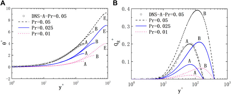
FIGURE 5. Non-dimensional temperature and heat flux of the plane for different Pr fluids. (A) temperature; (B) heat flux.

3.3 Numerical Analysis of the Square Bundle

To further analyze the applicability of the current isotropic four-equation model in complex geometries, the flow and heat of liquid metal with a Prandtl value of 0.01 in the quadrilateral infinite rod bundle were studied. Figure 6 shows the schematic diagram of the computational domain and local hexahedral mesh of the quadrilateral infinite rod bundle. Lines ab, bo, oc, and arc ca are the local distributions to be analyzed next. The flow parameters are reported in Table 4. The surfaces of rods in contact with the fluids are heated by uniform wall fluxes $q_w$. Symmetry condition is applied on other faces to simulate the infinite rod bundle region with a quadrilateral arrangement. The heat fully developed flow length $L_z$ is set to $10D_h$ (Ge et al., 2017). The rod diameter D and X = P/D ratio are the same as in Zhukov’s experiment (Zhukov et al., 2002).

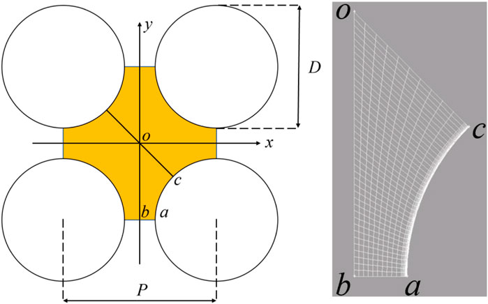
FIGURE 6. Schematic diagram of the quadrilateral infinite rod bundle. (A) flow area; (B) local mesh.

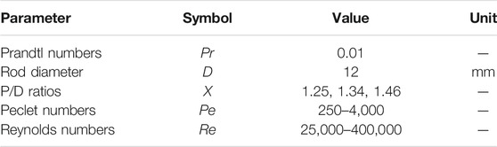
TABLE 4. Flow parameters.

3.3.1 Heat Transfer Evaluation and Analysis

In Table 5, a few important heat transfer correlations of Nusselt number $Nu$ are available for the quadrilateral infinite rod bundle, reviewed in the study by (Mikityuk 2009). Zhukov (Zhukov et al., 2002) obtained 36 Nu(Pe) data from the heat transfer experiment of 22%Na–78%K in a quadrilateral rod bundle. The correlations obtained by Subbotin (Subbotin et al., 1965) and BREST (Adamov 2001) were derived from triangular bundles, while Mikityuk, from a wide database, conducted experimental results of liquid metals (Mikityuk 2009). It is worth noting that there are no more available experimental data. The correlations should be used with care and be paid more attention to for analysis of the reliability. The $Nu$ can be calculated as follows:

where $n_i$ is a vector of a unit perpendicular to a sliced face.

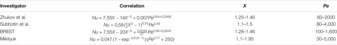
TABLE 5. Correlations of Nusselt number for the square bundle.

First, the simulations for $Pr$ = 0.01 are characterized by X = 1.25, 1.34, and 1.46 with a corresponding hydraulic diameter $D_h$ of 11.87, 15.43, and 20.57 mm. Nine simulations with bulk Reynolds numbers of 250–400,000 were operated. The corresponding Peclet number is approximately 250–4,000. Figure 7 shows the Nusselt number results for $X=1.25$ -1.46 cases. In Figure 7, Subbotin and Mikityuk correlations overestimated the Nusselt number compared with the conservative result of Zhukov and BREST. The correlation between these empirical relations is too poor to relate because these relationships have very different slopes.

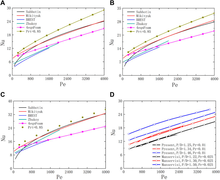
FIGURE 7. Schematic diagram of Nusselt number for the square bundle. (A) X = 1.25; (B) X = 1.34; (C) X = 1.46; (D) X = 1.22–1.5.

In Figures 7A–C, the prediction Nu of the isotropic $k-\tilde{\epsilon }-k_{\theta }-\widetilde{{\epsilon }_{\theta }}$ model almost lies between the experimental relationship. The prediction of the $P{r}_t=0.85$ model is higher than Subbotin and Mikityuk correlations. At low Peclet numbers, the $Nu$ results having a special slope predicted using the isotropic four-equation model is closer to the Subbotin and Mikityuk correlations, while the calculation results at high Pe are conservative, similar to the Zhukov and BREST correlations. The overall numerical Nu seems to be more conservative than these experimental correlations. Poor experimental relevance makes this problem’s numerical verification difficult to go on.

As shown in Figure 7D, the numerical slope in the Nu(Pe) line obtained using the $k-\tilde{\epsilon }-k_{\theta }-\widetilde{{\epsilon }_{\theta }}$ model is very similar to that predicted using Manservisi’s $k-\epsilon -k_{\theta }-{\epsilon }_{\theta }$ model, which has successfully predicted heat transfer calculation for $Pr=0.025$ fluids and can provide an additional CFD relationship reference. Therefore, we still use the present isotropic four-equation model for thermal analysis and local temperature calculations.

This present work focuses on the comparison of the effects of two turbulent thermal diffusion models (the $P{r}_t=0.85$ model and the present isotropic $k-\tilde{\epsilon }-k_{\theta }-\widetilde{{\epsilon }_{\theta }}$ model) on the temperature field, without considering the influence of different RANS turbulence $k-\epsilon$ or $k-w$ models. The detailed influence and performance evaluation of different turbulence models on liquid metal flow can be found in the literature (You et al., 2019).

3.3.2 Turbulent Thermal Fields

1) Coolant and wall temperature

Figure 8 shows the dimensionless temperature ${\theta }^{+}=\lambda (T-T_b)/(q_w·D_h)$ on a sliced surface of square bundle X = 1.25. The overall dimensionless temperature in the channel decreases with the increase in $Pe$. The temperature at the rod surface is not constant. The wall temperature near the center of the channels is lower than that near the center of gaps.

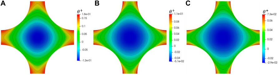
FIGURE 8. Schematic diagram of dimensionless temperature on a slice for square lattice X = 1.25. (A) Pe = 250; (B) Pe = 2000; (C) Pe = 4000.

Figure 6 has annotated the line ab, line bo, line oc, and arc ca, where points b and c represent the center of the gap and the channel, respectively. The dimensionless temperature field with Pe = 2000 is selected for analysis. In Figure 9A, with the decrease in P/D, the gap width decreases, and the overall dimensionless temperature distribution ${\theta }^{+}$ at the gap line ab increases. In Figures 9B,D, the coolant dimensionless temperature distribution from gap center point b to channel center point o and the wall dimensionless temperature distribution over arc ca are smoother in pace with strengthening of P/D. Due to the development of velocity and sufficient cooling of the fluid near the center of the channel, the dimensionless temperature distribution over line oc decreases when the value of P/D decreases in Figure 9C.

2) Fluctuation and isotropic dissipation

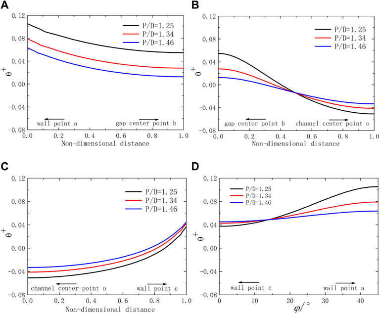
FIGURE 9. Schematic diagram of dimensionless temperature over lines for the square lattice at Pe = 2000 with different P/D ratios. (A) line ab; (B) line bo; (C) line oc; (D) arc ca.

The distribution and shape of $k_{\theta }$ and $\widetilde{{\epsilon }_{\theta }}$ for $Pe$ = 100, 2000, and 4,000 are shown in Figure 10. $k_{\theta }$ has a lower local value near the center point o. The maximum value appears near the wall. The maximum value of $k_{\theta }$ decreases when $Pe$ increases, while that of ${\epsilon }_{\theta }$ increases. The numerical shape and distribution of $k_{\theta }$ and its isotropic dissipation $\widetilde{{\epsilon }_{\theta }}$ obtained from the present $k-\tilde{\epsilon }-k_{\theta }-\widetilde{{\epsilon }_{\theta }}$ model is similar to that predicted by Manservisi’s $k-\epsilon -k_{\theta }-{\epsilon }_{\theta }$ model (Manservisi and Menghini, 2015). Further details on over line ab, line bo, and line oc can be found in Figure 11. The dimensionless root square means temperature ${\theta }_{rms}=\lambda \sqrt{2k_{\theta }}/\left(q{D}_h\right)$ is set. From wall point a to wall point b, ${\theta }_{rms}$ first increases to a small peak and then begins to decrease to point b. Then along the bo line, the maximum peak value of ${\theta }_{rms}$ is reached near the midpoint of the bo section. Three peaks of different sizes were formed on lines ab, bo, and oc, respectively. When it goes straight toward the wall point, it will eventually approach 0. When the value is $X$, the overall value of ${\theta }_{rms}$ decreases.

3) Turbulence and molecular thermal diffusivity

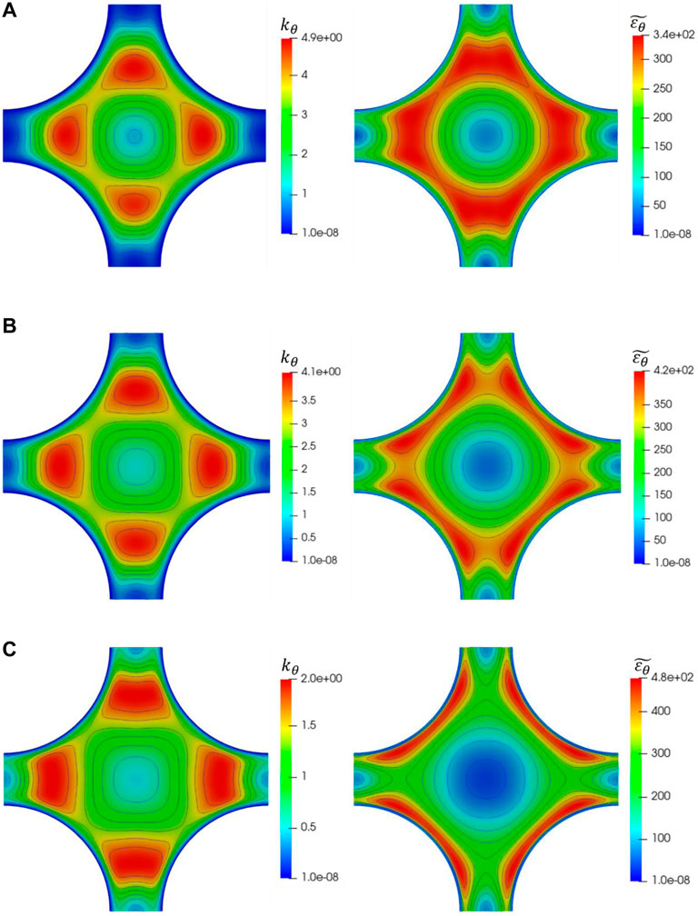
FIGURE 10. Schematic diagram of average temperature fluctuaion (left) and its isotropic dissipation (right) on a slice for square lattice X = 1.25. (A) Pe = 1000; (B) Pe = 2000; (C) Pe = 4000.

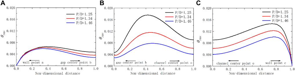
FIGURE 11. Schematic diagram of dimensionless temperature fluctuation over lines for the square lattice at Pe = 2000 with different P/D ratios. (A) line ab; (B) line bo; (C) line oc.

Figure 12 shows the proportional relationship of turbulent to molecular thermal diffusivity, that is, dimensionless thermal diffusivity $a^{+}={\alpha }_t/\alpha$, over line ab, line bo, and line oc with the change of $P/D$ for square bundle X = 1.25 at Pe = 2000. Reynolds heat flux $q_t$ and molecular heat flux $q_m$ can be defined as follows:

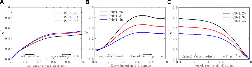
FIGURE 12. Schematic diagram of dimensionless thermal diffusivity over lines for the square lattice at Pe = 2000 with different P/D ratios. (A) line ab; (B) line bo; (C) line oc.

Thus, the specific value of turbulent to molecular thermal diffusivity represents the ratio of Reynolds to molecular heat flux. Reynolds heat flux is mainly caused by thermal diffusion caused by turbulent flow, while molecular heat conduction generates molecular heat flux. In Figure 12, in the area closest to the wall point a or c, $a^{+}$ tends to 0, which means turbulent heat diffusion tends to be ignored here. With the increase in wall distance from wall point a to gap center point b, the turbulent heat diffusion gradually increases, so the value of $a^{+}$ increases. However, $a^{+}$ is still less than one over line ab, which means that the molecular heat conduction of liquid metal always affects the heat transfer at the gap area. At the gap center point b, $a^{+}$ reaches a local maximum over line ab. It increases along the bo segment and reaches its maximum near the middle of the bo segment. In most regions far from the wall over lines bo and oc, due to the development of the turbulent flow, turbulent diffusion is greater than the molecular heat conduction, so $a^{+}>1$. Interestingly, the maximum value of $a^{+}$ does not appear at the channel center point o but near point o. At the gap line ab, the smaller the gap length, the greater the influence of molecular heat conduction, so the value of $a^{+}$ increases over the line ab when the valve of P/D increases. But it decreases over the line bo and line oc when the valve of P/D increases because at the same $Pe$, the larger the P/D, the larger the flow area, the smaller the overall velocity, and the smaller the turbulent heat diffusion over those areas. In Figure 13, the dimensionless thermal diffusivity on a slice for $Pe$ = 250, 1,000, 2000, and 4,000 is shown. At the same P/D, when the $Pe$ increases, turbulent heat diffusion will be enhanced, and the grid point with $a^{+}>1$ begins to appear.

4) Turbulent Prandtl number

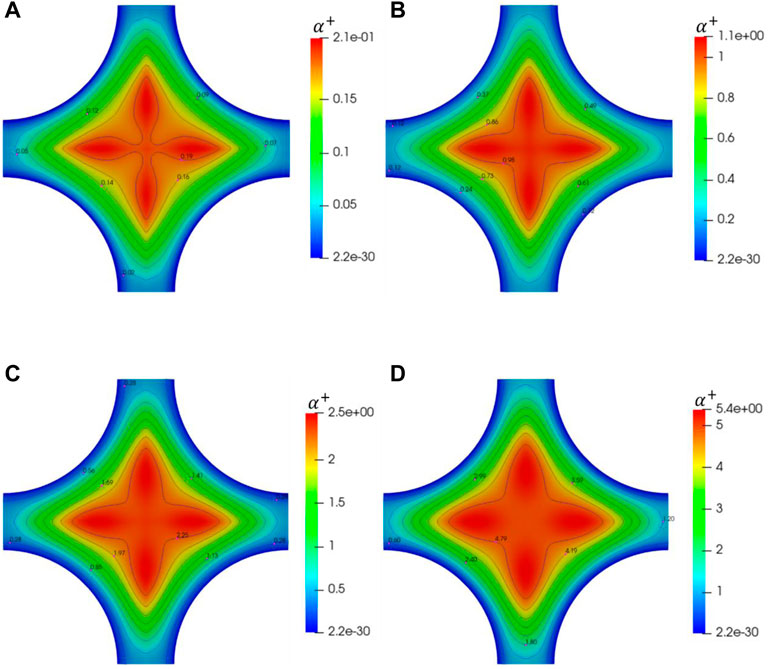
FIGURE 13. Schematic diagram of dimensionless thermal diffusivity on a slice for square lattice X = 1.25. (A) Pe = 250; (B) Pe = 1000; (C) Pe = 2000; (D) Pe = 4000.

In Figure 14, the Pr_t with the change of P/D is shown over the lines ab, bo, and oc for the square bundle with X = 1.25 at Pe =2000. The Pr_t is not constant and linear. It is larger than the general value of 0.85 for liquid metal. The Pr_t distribution on the line bo is to be smoother than that of lines ab and co. The value of Pr_t decreases over line ab when the value of P/D increases, while it increases over lines bo and oc. This phenomenon echoes the changing trend of dimensionless thermal diffusivity. In Figure 15, the turbulent Prandtl number on a slice for Pe = 1,000, 2000, and 4,000 for the square bundle is shown. When $Pe$ increases, Pr_t near the wall and the center decreases gradually.

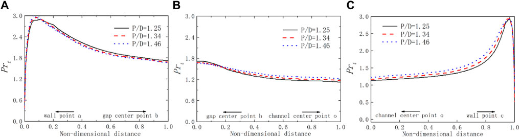
FIGURE 14. Schematic diagram of turbulent Prandtl number over lines for the square lattice at Pe = 2000 with different P/D ratios. (A) line ab; (B) line bo; (C) line oc.

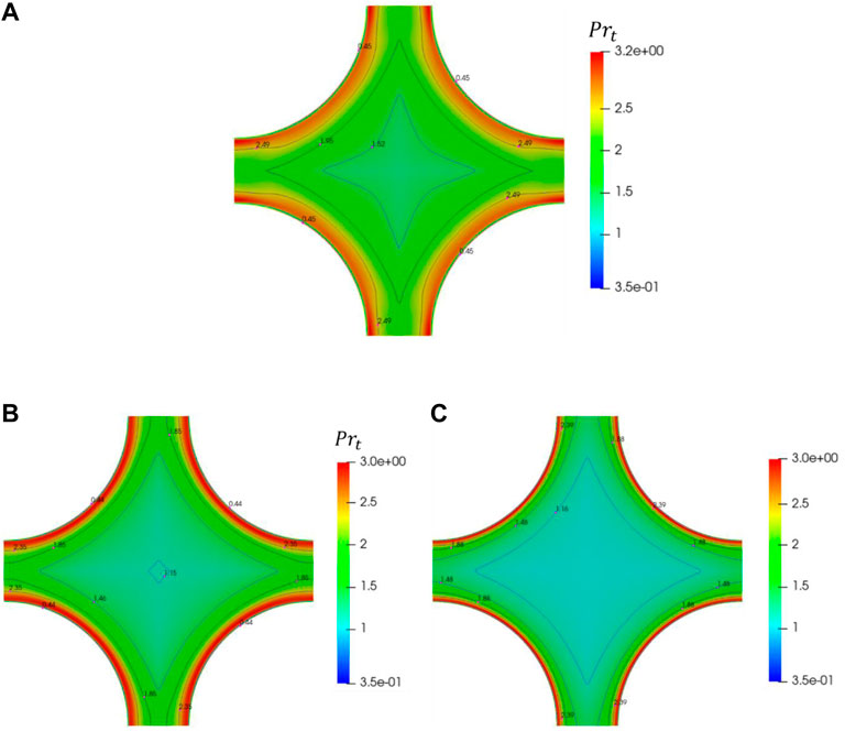
FIGURE 15. Schematic diagram of turbulent Prandtl number on a slice for square lattice X = 1.25. (A) Pe = 1000; (B) Pe = 2000; (C) Pe = 4000.

The average turbulent Prandtl number $P{r}_{tm}$ can be defined as follows:

Table 6 summarizes the calculation results of average turbulent Prandtl number $P{r}_{tm}$ under different P/D and Pe using the present $k-\tilde{\epsilon }-k_{\theta }-\widetilde{{\epsilon }_{\theta }}$ model. One can see that at the same P/D, the average turbulent Prandtl number decreases with the increase in Pe, while at the same Pe, it increases when the value of P/D increases.

5) Performance analysis of the present four-equation model

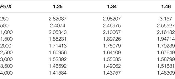
TABLE 6. Average turbulent Prandtl number under different P/D and Pe.

When the same turbulence $k-\tilde{\epsilon }$ model is kept to solve the turbulent viscosity, the present four-equation model needs to solve two more equations $k_{\theta }-\widetilde{{\epsilon }_{\theta }}$ than the Pr_t = 0.85 model. To analyze the calculation speed of the $k-\tilde{\epsilon }-k_{\theta }-\widetilde{{\epsilon }_{\theta }}$ model, the single-step iterative calculation time and calculation memory of these two models are compared and listed in Table 7. The current test platform is HP ProDesk 680 G⁴ MT with an Intel(R) Core(TM) i7-9700 CPU at 3.00 GHz and 16 GB system memory at 2,667 MHz. At present, the model solver is written based on OpenFOAM V6 version, compiled and integrated in Ubuntu 18.04 system environment. As shown in Table 7, the calculation time and memory required by the $k-\tilde{\epsilon }-k_{\theta }-\widetilde{{\epsilon }_{\theta }}$ model are greater than those of the $k-\tilde{\epsilon }-P{r}_t= 0.85$ model.

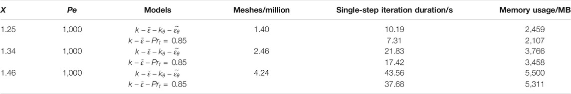
TABLE 7. Performance of the four-equation model under serial operation.

4 Conclusion

The present work studied an isotropic four-equation model for low Pr number that uses simple Dirichlet wall boundaries. First, the turbulent heat transfer process of Pr = 0.01 ∼ 0.05 fluid in the uniformly heated plane is numerically studied on the open-source program OpenFOAM. Then the flow and heat of the isotropic four-equation of the quadrilateral infinite rod bundle region are evaluated and analyzed with low Prandtl number Pr = 0.01. In the SGDH framework, the Pr_t = 0.85 model and the isotropic four-equation model are compared with available experimental correlations in the range of Pe = 250–4,000 and P/D = 1.25–1.46. The numerical results show that.

1) The full development velocity, temperature, Reynolds stress, and Reynolds heat flow of Pr = 0.01 ∼ 0.05 fluid in-plane predicted using the isotropic four-equation model are in good agreement with the DNS results.

2) The Nu of the isotropic four-equation model lies between the experimental relationship, more conservative and similar to the Zhukov and BREST correlations for square rod bundles, while the Pr_t = 0.85 model gives too high a Nusselt number prediction to predict the integra heat properly. The slope of Nu predicted by the present isotropic four-equation model is similar to Manservisi’s model.

3) More detailed heat exchange phenomena and local temperature distribution are obtained using the four-equation model. At the same P/D, the average turbulent Prandtl number decreases with the increase in Pe, while at the same Pe, it increases when the value of P/D increases.

The isotropic four-equation model can provide more references for calculating the thermal-hydraulic phenomena of liquid metals. But its wider applicability needs further verification.

Data Availability Statement

The raw data supporting the conclusion of this article will be made available by the authors, without undue reservation.

Author Contributions

XS: concept, research, writing, editing, code, and data processing. XL: modification, concept, research, and code. XW: research, modification, and code. YL: concept, editing, and research. QC: editing and research. QS: editing and research. XS: editing and research. GL: funding, project management, concept, and research.

Funding

This work was supported by the Research on key technology and safety verification of primary circuit, Grant No. 2020YFB1902104, and the Experimental study on thermal-hydraulics of fuel rod bundle, Grant No. Y828020XZ0.

Conflict of Interest

The authors declare that the research was conducted in the absence of any commercial or financial relationships that could be construed as a potential conflict of interest.

Publisher’s Note

All claims expressed in this article are solely those of the authors and do not necessarily represent those of their affiliated organizations, or those of the publisher, the editors, and the reviewers. Any product that may be evaluated in this article, or claim that may be made by its manufacturer, is not guaranteed or endorsed by the publisher.

References

Abe, K., Kondoh, T., and Nagano, Y. (1995). A New Turbulence Model for Predicting Fluid Flow and Heat Transfer in Separating and Reattaching Flows-II. Thermal Field Calculations. Int. J. Heat Mass Transfer 38 (8), 1467–1481. doi:10.1016/0017-9310(94)00252-q
Adamov, E. O. (2001). Naturally Safe Lead-Cooled Fast Reactor for LargeScale Nuclear Power. Moscow: Dollezhal RDIPE.
Cerroni, D., Da Vià, R., Manservisi, S., Menghini, F., Pozzetti, G., and Scardovelli, R. (2015). Numerical Validation of Aκ-ω-Κθ-Ωθheat Transfer Turbulence Model for Heavy Liquid Metals. J. Phys. Conf. Ser. 655 (1), 012046. doi:10.1088/1742-6596/655/1/012046
Cheng, X., and Tak, N.-i. (2006). Investigation on Turbulent Heat Transfer to lead-bismuth Eutectic Flows in Circular Tubes for Nuclear Applications. Nucl. Eng. Des. 236 (4), 385–393. doi:10.1016/j.nucengdes.2005.09.006
Chierici, A., Chirco, L., Da Vià, R., and Manservisi, S. (2019). Numerical Simulation of a Turbulent Lead Bismuth Eutectic Flow inside a 19 Pin Nuclear Reactor Bundle with a Four Logarithmic Parameter Turbulence Model. J. Phys. Conf. Ser. 1224, 012030. doi:10.1088/1742-6596/1224/1/012030
Choi, S. K., and Kim, S. O. (2007). Treatment of Turbulent Heat Fluxes with the Elliptic-Blending Second-Moment Closure for Turbulent Natural Convection Flows. Int. J. Heat Mass Transfer 51 (9-10), 2377–2388. doi:10.1016/j.ijheatmasstransfer.2007.08.012
Da Vià, R., Giovacchini, V., and Manservisi, S. (2020). A Logarithmic Turbulent Heat Transfer Model in Applications with Liquid Metals for Pr = 0.01-0.025. Appl. Sci. 10 (12), 4337. doi:10.3390/app10124337
Da Vià, R., and Manservisi, S. (2019). Numerical Simulation of Forced and Mixed Convection Turbulent Liquid Sodium Flow over a Vertical Backward Facing Step with a Four Parameter Turbulence Model. Int. J. Heat Mass Transfer 135, 591–603. doi:10.1016/j.ijheatmasstransfer.2019.01.129
Da Vià, R., Manservisi, S., and Menghini, F. (2016). A K-Ω-Kθ-Ωθ Four Parameter Logarithmic Turbulence Model for Liquid Metals. Int. J. Heat Mass Transfer 101 (10), 1030–1041. doi:10.1016/j.ijheatmasstransfer.2016.05.084
Deng, B., Wu, W., and Xi, S. (2001). A Near-wall Two-Equation Heat Transfer Model for wall Turbulent Flows. Int. J. Heat Mass Transfer 44 (4), 691–698. doi:10.1016/s0017-9310(00)00131-9
Duponcheel, M., Bricteux, L., Manconi, M., Winckelmans, G., and Bartosiewicz, Y. (2014). Assessment of RANS and Improved Near-wall Modeling for Forced Convection at Low Prandtl Numbers Based on LES up to Reτ=2000. Int. J. Heat Mass Transfer 75, 470–482. doi:10.1016/j.ijheatmasstransfer.2014.03.080
Ejenstam, J., and Szakálos, P. (2015). Long Term Corrosion Resistance of Alumina Forming Austenitic Stainless Steels in Liquid lead. J. Nucl. Mater. 461, 164–170. doi:10.1016/j.jnucmat.2015.03.011
Ge, Z., Liu, J., Zhao, P., Nie, X., and Ye, M. (2017). Investigation on the Applicability of Turbulent-Prandtl-Number Models in Bare Rod Bundles for Heavy Liquid Metals. Nucl. Eng. Des. 314, 198–206. doi:10.1016/j.nucengdes.2017.01.032
Groetzbach, G. (2013). Challenges in Low-Prandtl Number Heat Transfer Simulation and Modelling. Nucl. Eng. Des. 264, 41–55. doi:10.1016/j.nucengdes.2012.09.039
Gu, L., and Su, X. (2021). Latest Research Progress for LBE Coolant Reactor of China Initiative Accelerator Driven System Project. Front. Energ. 15, 810–831. doi:10.1007/s11708-021-0760-1
Kawamura, H., Abe, H., and Matsuo, Y. (1999). DNS of Turbulent Heat Transfer in Channel Flow with Respect to Reynolds and Prandtl Number Effects. Int. J. Heat Fluid Flow 20 (3), 196–207. doi:10.1016/s0142-727x(99)00014-4
Kawamura, H., Ohsaka, K., Abe, H., and Yamamoto, K. (1998). DNS of Turbulent Heat Transfer in Channel Flow with Low to Medium-High Prandtl Number Fluid. Int. J. Heat Fluid Flow 19 (5), 482–491. doi:10.1016/s0142-727x(98)10026-7
Kays, W. M. (1994). Turbulent Prandtl Number-Where Are We? Asme Trans. J. Heat Transfer 116 (2), 284–295. doi:10.1115/1.2911398
Lai, Y. G., and So, R. M. C. (1990). Near-wall Modeling of Turbulent Heat Fluxes. Int. J. Heat Mass Transfer 33 (7), 1429–1440. doi:10.1016/0017-9310(90)90040-2
Manservisi, S., and Menghini, F. (2014a). A CFD Four Parameter Heat Transfer Turbulence Model for Engineering Applications in Heavy Liquid Metals. Int. J. Heat Mass Transfer 69 (2), 312–326. doi:10.1016/j.ijheatmasstransfer.2013.10.017
Manservisi, S., and Menghini, F. (2015). CFD Simulations in Heavy Liquid Metal Flows for Square Lattice Bare Rod Bundle Geometries with a Four Parameter Heat Transfer Turbulence Model. Nucl. Eng. Des. 295 (12), 251–260. doi:10.1016/j.nucengdes.2015.10.006
Manservisi, S., and Menghini, F. (2014b). Triangular Rod Bundle Simulations of a CFD κ-ϵ-κ-ϵ Heat Transfer Turbulence Model for Heavy Liquid Metals. Nucl. Eng. Des. 273, 251–270. doi:10.1016/j.nucengdes.2014.03.022
Mikityuk, K. (2009). Heat Transfer to Liquid Metal: Review of Data and Correlations for Tube Bundles. Nucl. Eng. Des. 239 (4), 680–687. doi:10.1016/j.nucengdes.2008.12.014
Moukalled, F., Mangani, L., and Darwish, M. (2016). The Finite Volume Method in Computational Fluid Dynamics. Berlin: Springer International Publishing.
Nagano, Y., Hattori, H., and Abe, K. (1997). Modeling the Turbulent Heat and Momentum Transfer in Flows under Different thermal Conditions. Fluid Dyn. Res. 20 (1-6), 127–142. doi:10.1016/s0169-5983(96)00049-4
Nagano, Y., and Kim, C. (1988). A Two-Equation Model for Heat Transport in Wall Turbulent Shear Flows. J. Heat Transfer 110 (3), 583–589. doi:10.1115/1.3250532
Nagano, Y., and Shimada, M. (1996). Development of a Two‐equation Heat Transfer Model Based on Direct Simulations of Turbulent Flows with Different Prandtl Numbers. Phys. Fluids 8 (12), 3379–3402. doi:10.1063/1.869124
Reynolds, A. J. (1975). The Prediction of Turbulent Prandtl and Schmidt Numbers. Int. J. Heat Mass Transfer 18 (9), 1055–1069. doi:10.1016/0017-9310(75)90223-9
Schroer, C., Wedemeyer, O., Skrypnik, A., Novotny, J., and Konys, J. (2012). Corrosion Kinetics of Steel T91 in Flowing Oxygen-Containing lead–bismuth Eutectic at 450 °C. J. Nucl. Mater. 431 (1-3), 105–112. doi:10.1016/j.jnucmat.2011.11.014
Shams, A., De Santis, A., and Roelofs, F. (2019). An Overview of the AHFM-NRG Formulations for the Accurate Prediction of Turbulent Flow and Heat Transfer in Low-Prandtl Number Flows. Nucl. Eng. Des. 355, 110342. doi:10.1016/j.nucengdes.2019.110342
Shikazono, N., and Kasagi, N. (1996). Second-moment Closure for Turbulent Scalar Transport at Various Prandtl Numbers. Int. J. Heat Mass Transfer 39 (14), 2977–2987. doi:10.1016/0017-9310(95)00339-8
Su, X. K., and Gu, L. (2021). Numerical Study on Turbulent Heat Transfer of LBE in an Annulus Based on A Four-Equation Model. Chinese Beijing: Atomic Energy Science and technology. Avaialbe at: http://kns.cnki.net/kcms/detail/11.2044.TL.20210720.181. doi:10.13832/j.jnpe.2021.S1.0026
Su, X. K., Gu, L., Peng, T. J., Jiatai, L., Xianwen, L., and Guan, W. (2021). Research on a Four-Equation Model Based on OpenFOAM. Nucl. Power Eng. 42 (S1), 26–32. (in chinese).
Subbotin, V. I., Ushakov, P. A., and Kirillov, P. L. (1965). “Heat Transfer in Elements of Reactors with a Liquid Metal Coolant,” in Proceedings of the 3rd International Conference on Peaceful Use of Nuclear Energy, Geneva, 192–200.
Tiselj, I., and Cizelj, L. (2012). DNS of Turbulent Channel Flow with Conjugate Heat Transfer at Prandtl Number 0.01. Nucl. Eng. Des. 253 (1), 153–160. doi:10.1016/j.nucengdes.2012.08.008
Wang, G., Gu, L., and Yun, D. (2021). Preliminary Multi-Physics Performance Analysis and Design Evaluation of UO2 Fuel for LBE-Cooled Subcritical Reactor of China Initiative Accelerator Driven System. Front. Energ. Res. doi:10.3389/FENRG.202110.3389/fenrg.2021.732801
Weller, H. G., Tabor, G., Jasak, H., and Fureby, C. (1998). A Tensorial Approach to Computational Continuum Mechanics Using Object-Oriented Techniques. Comput. Phys. 12 (6), 620–631. doi:10.1063/1.168744
You, B. H., Jeong, Y. H., and Addad, Y. (2019). Assessment of Advanced RANS Models Ability to Predict a Turbulent Swept Liquid Metal Flow over a Wire in a Channel. Nucl. Eng. Des. 353 (Nov), 1102061–11020614. doi:10.1016/j.nucengdes.2019.110206
Youssef, M. S. (2006). A Two-Equation Heat Transfer Model for wall Turbulent Shear Flows. J. Eng. Sci. 34 (6), 1877–1903. doi:10.21608/jesaun.2006.111184
Keywords: low Pr fluid, four-equation, OpenFOAM, heat transfer, liquid metal
Citation: Su X, Li X, Wang X, Liu Y, Chen Q, Shi Q, Sheng X and Gu L (2022) Development and Assessment of an Isotropic Four-Equation Model for Heat Transfer of Low Prandtl Number Fluids. Front. Energy Res. 10:816560. doi: 10.3389/fenrg.2022.816560
Received: 16 November 2021; Accepted: 14 January 2022;
Published: 08 February 2022.
Edited by:
Wei Ding, Helmholtz Association of German Research Centres (HZ), GermanyReviewed by:
Yacine Addad, Khalifa University, United Arab EmiratesLuteng Zhang, Chongqing University, China
Copyright © 2022 Su, Li, Wang, Liu, Chen, Shi, Sheng and Gu. This is an open-access article distributed under the terms of the Creative Commons Attribution License (CC BY). The use, distribution or reproduction in other forums is permitted, provided the original author(s) and the copyright owner(s) are credited and that the original publication in this journal is cited, in accordance with accepted academic practice. No use, distribution or reproduction is permitted which does not comply with these terms.
*Correspondence: Long Gu, gulong@impcas.ac.cn