Assessment of the Impact of Higher Temperatures Due to Climate Change on the Mortality Risk Indexes in Ecuador Until 2070

Introduction

Climate change (CC) is a fundamental issue for humanity, representing a threat to the natural resources and systems upon which we rely on. Changes in climate conditions are due to natural factors, e.g., atmospherics and oceanic mechanisms, and changes in natural cycles (IPCC. et al., 2014). However, the high global mean temperature increases in the last century in relation to preindustrial values are unprecedented and certainly related to anthropogenic activities. The range in global surface temperature has increased from 1850 to 1900 to 2010–2019 from 0.8°C to 1.3°C (IPCC, 2021), and the projected temperature shows an increase between 1.8°C and 5.8°C by 2,100 (Haines & Patz, (2004). In addition, sea levels are projected to rise between 9 and 88 cm during the next century, with accompanied changes in sea salinity (Heuzé et al., 2013), and higher intensity and frequency of occurrence of heat waves and tropical cyclones (Steffen et al., 2014). Indeed, it is critical that we enhance our knowledge of the local effects and impacts associated with climate change in order to develop contextual and novel strategies to mitigate and adapt to climate change in our region (Mach et al., 2016; Pasqui and Di Giuseppe, 2019).

The surface temperature shows an increase worldwide (Mach et al., 2016) in scenarios of CC; however, it is not homogenous across the regions. For instance, Sa’adi et al. (2020) displays the minimum temperature projected to increase more (3.3–4.7°C) compared with maximum temperature (3.0–4.6°C) in Borneo Island from CMIP5 models. Also, Zhou et al. (2018), found an increased temperature pattern over Canadian Prairies derived from CMIP5 models. Moreover, Ongoma et al. (2018) projected East Africa to warm by 1.7°C–2.7°C and 2.2°C–5.4°C under RCP 4.5 and RCP 8.5 scenarios respectively in the last half of the 21 century. Wang et al. (2014), projected an increase of temperature by 0.8–1.6°C (0.8–1.7°C), 1.5–2.7°C (2°C–3.7°C), and 1.9°C–3.3°C (3.4°C–6°C) under RCP 4.5 (RCP 8.5) in three time slices (2010–2039, 2040–2069, and 2070–2099), respectively, over southwest China. Finally, Rusticucci and Zazulie (2021) show an increase in several temperature indices from CMIP5 models over South America. The projection of temperature will vary according to the models and climate scenario chosen; thus, it is important to evaluate the changes in regional temperature.

Worldwide, there is evidence of CC impacts on human health with an increase in mortality risks (Limaye et al., 2018; Morefield et al., 2018; Patz et al., 2005; Song et al., 2021). Changes in global temperature result in an increase in heat extremes, such that more stress episodes are expected at both global and regional scales (Seneviratne et al., 2014; Stott et al., 2016). In fact, older people have higher vulnerability when heat–cold waves are observed (Worfolk, 2000; Kovats and Hajat, 2008). Although, the link between extreme temperatures and indoor comfort has been widely studied (Lozano and Siegel, 2018; Schweiker et al., 2019), the understanding of the relationship between heat–cold temperature waves and heat stress (HS) is complex (Kyselý, 2004; Anderson and Bell, 2009; Montero et al., 2012). In particular, this remains a challenge in developing countries because data of HS and mortality rates are scarce.

There are several methodologies to evaluate HS. Sherwood and Huber (2010) combined daily temperatures and humidity into a single metric to measure HS; thus, a wet bulb temperature above 35°C for long periods should have negative incidences on the health of humans and mammals. Matzarakis et al. (1999) proposed the physiological equivalent temperature index, which derives from the human energy balance. On the other hand, Shi et al. (2015) argued that increasing standard deviation of daily temperatures during summer and winter is harmful, leading to a rise in mortality in warmer summers.

Another open area of research is the assessment of the heat index approach for associating HS and mortality rates using data from weather stations in terrain. Christidis et al. (2019) proposed a novel methodology, assuming the V-shaped model developed by Honda et al. (2007) where the 84th percentile of the maximum daily temperature (Tmax) is assumed as the optimum temperature (OT) for some areas in Japan, related to the lowest mortality rates. Thus, temperatures either above or below the OT show an increase in mortality rates. Afterward, Honda et al. (2014) conveyed a similar study to evaluate the V-shaped model worldwide. They found that the 84th percentile of the Tmax is a good estimator of OT not only in Japan but also in other cities with different climates such as Seoul, Phoenix, Paris, and Barcelona.

Using the V-shaped model, Christidis et al. (2019) assume that the 84th percentile of the daily Tmax is a good estimator of OT globally, including South America, suggesting that the metabolism of people needs some period to adapt to an increase in the number of days above the OT observed in the natural period, i.e., the period prior to industrialization. However, the increase in warming days above the OT due to CC conditions could induce HS to people. In order to determine the health impact of CC, Christidis et al. (2019) introduced two indices, namely, 1) high risk warming (HRW) and 2) high risk days (HRD) that enable quantifying the effects of the intensity and frequency of heat waves. During the last 6 decades, the increase in temperature has been evident worldwide. For instance, Ecuador showed an intense warming trend in the 1966–2011 period (Morán-Tejeda et al., 2016). Thus, the projection of HS derived from IPCC CC scenarios may help to evaluate the future trends of heat-related mortality risk.

The climate of Ecuador is zoned into three main climatic regions (Ballari et al., 2018), which are influenced by the intertropical convergence zone (ITCZ), the Amazon perturbations, the Peruvian trough (Chimborazo and Vuille, 2021), the Southeastern Pacific Semipermanent High, and the well-known Caribbean High (Lockwood, 2009). In addition, El Niño Southern Oscillation (ENSO) is one of the predominant sources of interannual climate variability (Francou et al., 2004; Vuille and Werner, 2005) and produces above/below normal precipitation and temperature during El Niño/La Niña periods on the coast, while generating opposite conditions in the Andes and the Amazon. In Ecuador, the CMIP5 models project a decrease in drought by 2070 (Campozano et al., 2020); however, the temperature projections of these models have not yet been analyzed. On the other hand, based on the CMIP3 models, Buytaert et al. (2010) found that temperature projections display an average increase of 3°C in Ecuador toward the end of the century for the A₁B emission scenario. However, the effects of the incidence of extreme heating events due to CC conditions upon health and mortality risk has not been assessed in Ecuador. Despite its importance, research related to this urgent issue is limited in the Latin American region (Ebi et al., 2020).

This study aims to evaluate the impact of the increase in temperature due to CC on the mortality rate risk in Ecuador, assuming that Honda’s “V-shaped” model is valid in this country across its diverse climatic regions. Thus, the mortality risk is assessed by evaluating the future HRW and HRD trends for the period 2011–2070 in Ecuador in relation to the base period 1980–2005. Dynamical downscaled data to 10 km resolution, from three CMIP5 models, e.g., CSIRO-MK36, GISS-E2, and IPSL-CM5A-MR were used to improve the spatial representation of daily maximum temperature. This study serves as a stepping stone for adaptation strategies to reduce the temperature-related mortality and morbidity risks.

Materials and Methods

Study Area

The study area is continental Ecuador (area 256.370 km²), over the equatorial line in South America, whose climate is mostly defined by the Andean mountains acting as a weather divide (Bendix and Lauer, 1992). There are three natural regions in continental Ecuador, namely, the Coast region next to the Pacific Ocean, the Andes over the Andean Mountain, and the east Amazon region (Figure 1A). The wet season is related to the intertropical convergence zone (ITCZ) wherein warm air masses cover the Coastal region, characterized by rainfall and high temperature rise. In the opposite, the ITCZ displacement and the equatorial front result in the presence of cooler and drier air masses covering the southwestern region, which contribute to the dry season (Goldberg et al., 1987; Bendix and Lauer, 1992; Campozano et al., 2016). The Andes shows a larger spatial variability of the air temperatures, mainly associated to the topography of this specific region (Navarro-Serrano et al., 2020), and explained by sea surface temperature anomalies of Regions 3.4 and 3 of the El Niño Southern Oscillation (ENSO) (Vicente-Serrano et al., 2017). The temperature in the north of the Andes is a response to the North Atlantic SSTA (Vuille et al., 2000). The Amazon region has mean temperature values of 20.82°C with a standard deviation of 4.49°C (Moura et al., 2019).

FIGURE 1. (A) Location of Ecuador in South America and (B) location of temperature gauges; shape of labels denotes different climate zones (square, Coast; circle, Andes; triangle, Amazon), and it shows the 84th percentile of daily maximum temperature (P84Tmax) in Ecuador from the historical period (1981–2005); temperature is expressed in degrees Celsius.

During the historical period (NAT) between 1981 and 2005 in Ecuador, models show a high, the 84th percentile of the maximum temperature (P84Tmax) between 27°C and 33°C in the Coast, a variability of the P84Tmax between 16°C and 27°C in the Andes, and between 27°C and 33°C in the Amazon region (Figure 1B). In the Andes, the temperature variability is high between gauges, which could be associated to altitude. The inverse altitude–temperature is observed. In the Coast and Amazon, the temperature is in the range from 27°C to 33°C, evidencing their lower elevation.

Temperature In situ Observation

Daily observations of maximum temperature of 23 stations were provided by the Instituto Nacional de Meteorología e Hidrología de Ecuador (INAMHI). The location of the gauges is shown in Figure 1B. Due to limited data availability, the time period between January 1981 and December 2005 was considered as the base period, called natural period by Christidis et al. (2019). The stations with more than 10% of missing data were discarded; also, the homogeneity of the data was checked. The missing data were filled using random forest methods developed by Stekhoven and Bühlman (2012).

Global Climate Models

The CSIRO-MK36, GISS-E2, and IPSL-CM5A-MR global climate models (GCM) from the CMIP5 World Research Programme, dynamical downscaled to 10 km × 10 km, using the Weather Research and Forecasting model, WRF version 3.6.1, published in the Third National Communication of Ecuador (Table 1), were used for present and future maximum temperatures. These models were selected among 42 available models realized by Armenta et al. (2016), based on statistical metrics from several stations in the whole country. The models have different original resolution (see Table 1), and after a sensibility study, the following parametrizations were applied: Microphysics WSM 3-class simple ice; short-wave radiation, rapid radiation transfer model (rrtm); long-wave radiation, Dudhia; surface layer, Monin–Obukhov; land surface model, unified Noah land-surface model; boundary layer, YSU (Yonsei University) and Kain–Fritsh (new Eta) for cumulus parameterization (Armenta et al., 2016). After the downscaling process was conveyed, the maximum daily temperature was extracted from NetCDF files. The data were taken from the pixel closer to each ground station. From now on, the WRF downscaled GCM data will be named WGCM.

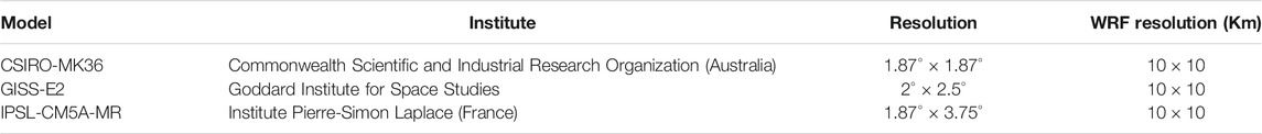
TABLE 1. Models used in this study.

To contribute with a more informed based decision making, the projections for the periods 2011–2040 and 2041–2070 were considered. Looking at mid-century and sooner, RCP 8.5 is clearly the most useful choice (Chaturvedi et al., 2012), which is a high-emission scenario with a prescribed 8.5-Wm^-2 radiative forcing, showing a high increase in greenhouse gas emission rate (Hibbard et al., 2011). RCP 8.5 describes a worst-case and plausible future scenario attributed to high population grown and minimal efforts to control energy demand ((Riahi et al., 2007); (Riahi et al., 2011)). Also, the RCP 8.5 is considered as highly relevant within in a short time horizon for decision making (2050) because it is in close agreement with historical total cumulative CO₂ emissions (Schwalm et al., 2020); thus, it is identified as business as usual scenario. Complementarily, RCP 8.5 projections show the highest increase in future temperature, which may imply higher temperature-related mortality risks.

Correction of Downscaled Temperature Projections

The analysis of historical temperature in Ecuador was conducted in the NAT, and the comparison between in situ observations and 10-km resolution WGCM data was carried out through the mean absolute error (MAE) and root mean square error (RMSE). Afterward, the simulations by WGCM data were corrected using empirical adjustment of variables by quantiles, using the library QMAP (Gudmundsson et al., 2012). Once the WGCM data are corrected in the present using an optimal bias correction function, such correction is applied to the WGCM in the future.

QMAP uses the distribution-derived transfer function to adjust the distribution of a modeled variable (Pm) so that it matches the distribution of an observed variable (Po). The distribution-derived transfer function is defined by Piani et al. (2010).

Statistical transformations are an application of the probability integral transform (Angus, 1994) to the known distribution of the variable of interest. The transformation is defined as:

where Fm is a CDF, and Fo⁻¹ is the corresponding quantile function (inverse CDF). The subscripts o and m indicate distribution parameters that correspond to observed and modeled data, respectively. For more details, we refer the reader to Gudmundsson (2016).

The quantile–quantile transformation using QMAP (Gudmundsson, 2012) has several options. In this study, the following were applied and its performance evaluated using the mean absolute error. Thus, the following transformation was analyzed:

The power transformation function

The relation quantile–quantile can be modeled using power transformation with the following equation:

where $\widehat{Po}$ indicates the best estimate of $Po$. The simple scaling (Eq. 3) is regularly used to adjust data from the regional climate model (see (Maraun et al., 2010)).

Empirical Quantiles (QUANT and RQUANT)

In order to solve Eq. 2 following the procedure by Boé et al. (2007), the empirical CDFs are approximated using tables of the empirical percentiles for QUANT. Values in between the percentiles are approximated using linear interpolation (Gudmundsson et al., 2012). Furthermore, RQUANT estimates the values of the quantile–quantile relation of the observed and modeled data for regularly spaced quantiles using local linear least square regression.

Smoothing Splines (SSPLIN)

The transformation of Eq. 1 can be solved using nonparametric regression (Gudmundsson et al., 2012). Thus, for the parametric transformation, the smoothing spline is only fitted to the fraction of the CDF corresponding to observed days. The smoothing parameter of the spline is identified by means of generalized cross-validation.

High-Temperature Mortality-Related Indices

High Risk Warming

In this study, the main assumption is that the optimum temperature (OT) with respect to the minimum mortality can be well represented by the 84th percentile of the Tmax for a given year (P84Tmax). This hypothesis was proposed by Honda et al. (2007, 2014) and supported by Zeng et al. (2016). Thus, based on this assumption, the high risk warming (HRW) index was developed by Christidis et al. (2019). This index measures the excess of P84Tmax for a given year i, with respect to P84Tmax of the natural period. In this study, the natural period is considered from 01–1981 to 12–2005. The HRW is expressed by Eq. 3 (Christidis et al., 2019).

where $HR{W}_{yri}$ is the HRW for the year i, $Tmax84\left(yri\right)$ is the 84th percentile of year i, and $Tmax{84}_{NAT}$ is the maximum temperature 84th percentile natural period. The evaluation of the future $HR{W}_{yri}$ was conducted for two futures periods, 2011–2040 and 2031–2070 for a better interpretation.

High Risk Days

The high risk day (HRD) index relates the number of days for a given year in the future over the P$Tmax{84}_{NAT}$. This index quantify the increase in the risk of mortality related to the increase in the number of days where humans were adapted ((Christidis et al., 2019). The HRD is calculated using Eq. 4.

where $HR{D}_{yri}$ is the HRD for a $yri$ in the future, $N{D}_{NAT}$ is the mean number of days above P84Tmax in the natural period, and $Nf\left(yri\right)$ is the number of days for a given year in the future above of $Tmax{84}_{NAT}$.

Analysis of the Trends of Heat-Related Indices

Projections have to be interpreted as the stochastic occurrence of a variable for a given period. It means that a specific value for a given year cannot be considered as forecasting data for this year. Thus, to have a better interpretation, for instance, the mean value, the variance, or the trend may be useful to evaluate such projections. In this study, two models were used for analyzing the trends of HRW and HRD. First, the Mann–Kendall trend model (MKTM) enables to determine the trend and its significance. Second, the Sen’s slope test (SST) was used to determine the magnitude of the variation in each region, namely, Coast, Andes, and Amazon.

Mann–Kendall Trend Model

In the MKTM, the S is calculated using the formula that follows:

where $T_j$ and $T_i$ are the annual values in years j and $i$, and $n$ is the number of data points. The value of $Sign\left(T_j-T_i\right)$ is calculated as follows:

This statistic presents the number of positive differences minus the number of negatives differences for all differences considered.

Thus, the variance $Var\left(S\right)$ is calculated as:

where $n$ is the number of data points, m is the number of tied groups, and $T_i$ is the number of ties extent i. Also, where the sample size is $n>10$, the standard test statistic Zs is computed as follows in Eq. 9:

Positives values of $Zs$ represents an increase tendency, while negative $Zs$ values show a decreasing trend. Thus, the MKTM is a nonparametric model widely used to find the trend in hydrometeorological time series (e.g., Vogel and Kroll, 2000; Modarres et al., 2007).

Sen’s Slope Estimator Test

Sen’s slope estimator test (SST) has been extensively used to determine the magnitude of the trend of the time series (Yue and Hashino, 2003; Yunling and Yiping, 2005; Tabari et al., 2011). The slope for all data pairs is calculated as (Sen, 1968):

Thus, in Eq. 10, $Q_t$ is the slope, $B$ is a constant, and $t$ is time. In order to determine $Q_t$, the follows equation is used:

In Eq. 11, $i=\mathrm{1,2,3},\dots$ N, whereas at time $j$ and $k$ $(j>k)$, $xj$ and $xk$ are the values of the data pairs. Therefore, the median ($Q_{med}$) of $N$ values of $Ti$ has been expressed as the SST, given as:

In addition, $Q_{med}$ is calculated to obtain the trend and slope magnitude by means of the nonparametric model. Thus, an upward trend is assumed when $Q_i$ is positive, whereas a downward trend is assumed when $Q_i$ is negative; finally, values closer to zero indicate no trend in the time. The units of SST would be slope magnitude in original units per year or percent per year (Salmi, 2002). Consequently, the HRW and HRD series were examined through MKTM and SST, to determine the trends and their magnitude, respectively.

Results

Correction of Present and Future Daily Maximum Temperature

In order to reduce the bias, four quantile-based correction methods, e.g., PTF, RQUANT, QUANT, and SSPLIN, were tested (see Gudmundsson et al., 2012). For evaluation purposes, the MAE was calculated for WGCM, with and without correction. Thus, CSIRO, GISS, and IPSL without corrections achieved MAE means of 2.99, 3.04, and 3.07, respectively (Table 2). After of the corrections, the models show a decrease in the MAE, and the temperature is closer to the observations; these values of MAE are very similar to each other, specifically RQUANT, QUANT, and SSPLIN achieved a MAE of 2.20 for CSIRO, 2.24 for GISS, and 2.28 for IPSL. On the other hand, PTF shows the lowest MAE values, which are 2.16, 2.21, and 2.16 for the CSIRO, GISS, and IPSL models.

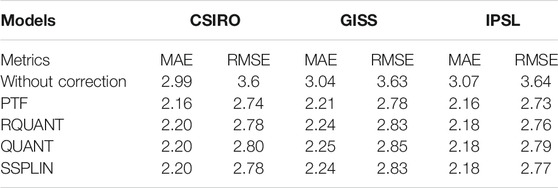
TABLE 2. Mean of mean absolute error (MAE) and root mean square error (RMSE) without correction and with correction through four different methods.

Thus, the models without bias correction exhibit a large difference between simulated and observed data (Figures 2A–C). However, CSIRO, GISS, and IPSL show a similar overestimation between 0°C and 4°C in the Coast. Over the Andes, the three models show the largest overestimation and underestimation between 0°C and 8 °C and between 0°C and −4°C, respectively. These facts highlight the complexities related to temperature variability for strong orographic gradients in mountain regions. Finally, in the Amazon, the overestimation is between 0°C and 2°C for CSIRO and IPSL, and for GISS, the difference is between 0°C and 4°C, which is the largest bias in the Amazon. After the corrections, the differences between observed and simulated temperatures are small, and the models show very similar spatial differences from −2°C to 2°C, achieving a greater bias reduction with respect to the models without correction (Figures 2D–F). To improve the forecasts, the same correction used in NAT was applied for the future. Thus, given the best performance of PTF quantile correction in the NAT period, station-wise parameters of PTF were applied for the future in all WGCMs.

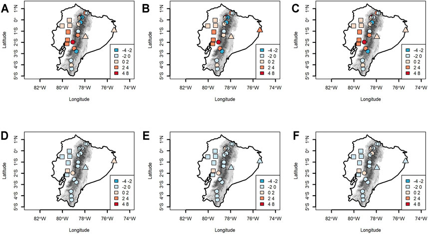
FIGURE 2. Differences between simulated and observed P84Tmax values. In columns are the models CSIRO, GISS, and IPSL. In the rows; without correction models (A–C) and corrected models through PTF method (D–F).

Spatial and Temporal Analysis of High Risk Warming and High Risk Day in Representative Concentration Pathway 8.5

High Risk Warming

Figure 3 displays plots of the mean of HRW for the 2011–2040 period. This period shows an increase in HRW between 0.6°C and 1.4°C. The CSIRO model exhibits the larger changes in the Coast, Amazon, and south of the Andes. The lowest change occurs over the central and northern Andes (Figure 3A). The GISS model displays an HRW increase in the 2011–2040 period; this change is heterogeneous over the three climate zones (Figure 3B), namely, an increase from 0.6°C to 1.2°C in the Coast, the higher rise from 0.6°C to 1.4°C in the Andes, and from 0.9°C to 1.2°C in the Amazon. The HRW derived from the IPSL model exhibits the lowest rises, which are between 0.6°C and 0.9°C in the Coast, between 0.9°C and 1.2°C in the Andes, and the forecast highest rise between 1.2°C and 1.4°C in the Amazon (Figure 3C). Finally, the ensemble shows, in all temperature gauges, an increase in HRW between 0.6°C and 1.2°C (Figure 3D).

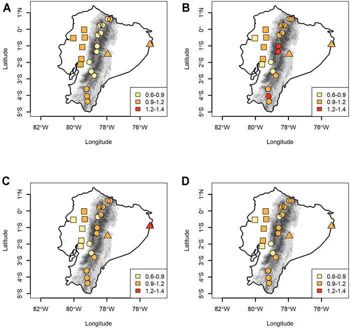
FIGURE 3. High risk warming (HRW) mean value for the period 2011–2040 from CSIRO (A), GISS (B), and IPSL (C). Figure 3D is the ensemble that explains the median from three WGCMs.

Figure 4 shows the mean of HRW for the period 2041–2070, in which the effects of the CC show a high increase. Specifically, the CSIRO model shows an HRW between 2.7°C and 3.6°C over the Coast region (Figure 4A), an increase between 1.8°C and 2.7°C in the north of the Andes, and from 2.7°C to 3.6°C in the south. In the Amazon, the expected rise is between 3.4°C and 4.6°C. The GISS model displays an increase in HRW in all regions, with rises between 1.6°C and 3.6°C; the highest increases are reported in some station in the Andes (Figure 4B). The IPSL model shows the highest values, which are heterogenous in all regions: the rise in HRW is between 1.8°C and 2.6°C in the Coast, Andes, and the Amazon; the boost is between 2.7°C and 3.6°C. Finally, the ensemble shows, in all temperature gauges, an increase in HRW between 1.8°C and 4.6°C (Figure 4D).

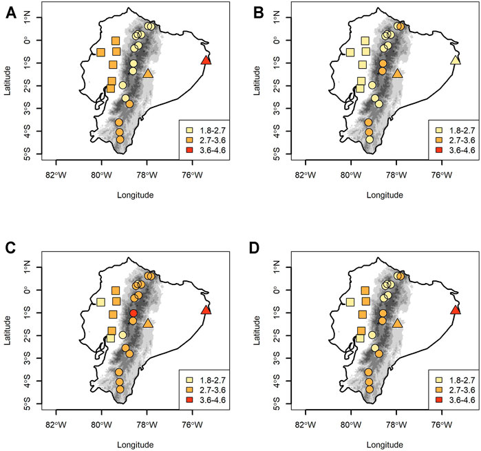
FIGURE 4. HRW mean value for the period 2041–2070 from CSIRO (A), GISS (B), and IPSL (C). Figure 4D is the ensemble that explains the median from three WGCMs.

HRW was calculated in every station for a year, and averages of all stations were plotted for every year (Figure 5). The CSIRO model shows a growing trend, namely, for 2040, the HRW is between 1.5°C and 2°C, and for 2070, it shows a strong increase around 3° (Figure 5A). The HRW peaks are persistent in time, varying between −1.5°C and 4.5°C. In Ecuador, the HRW obtained from the GISS model shows increases and decreases in the period 2011–2040. The variation is high every year, with peaks of +4 and −1°C; however, from 2045, the peaks are less frequent, and a steady increase is observed in HRW (Figure 5B). For 2070, an increase of 3°C is observed in all Ecuador. Figure 5C describes a growing trend for the HRW obtained from the IPSL model. The peaks are from −1°C to +2.5°C for 2011–2040, and for 2041–2070, the trend continues growing with peaks between +1°C and +4.5°C; these peaks are small relative to the other model. The growing trend is steeper, and the estimated HRW increase for 2070 is above 4°C. The ensemble shows, in all temperature gauges, an increase in HRW between 1°C and 2°C for 2011–2040 and for 2041–2070 peaks between 2°C and 4°C (Figure 5D).

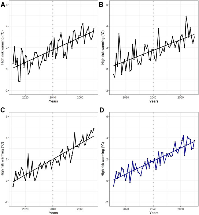
FIGURE 5. HRW of temperature gauges in Ecuador from CSIRO (A), GISS (B), and IPSL (C). Figure 5D is the ensemble that explains the median from three WGCMs. Values of the HRW axis are between −2°C and 6°C.

High Risk Days

Figure 6 displays plots of the mean of HRD for the 2011–2040 period. The HRD presents an increase from 52 to 74 days in the Coast, while in the Andes, the spatial pattern is heterogeneous with an increase from 42 to 62 days with CSIRO, and in the Amazon, the trend grows from 52 to 62 days (Figure 6A). The HRD from GISS shows lower changes, specifically between 42 and 52 days in the Coast and south of the Andes, and between 52 and 62 days in the north of the Andes and Amazon (Figure 6B). The HRD from IPSL exhibits a higher increase in all regions, mainly in the north of Andes where the rise is from 62 to 74 days, whereas in the Coast, the increase is between 42 and 74 days and in the Amazon, it is between 52 and 62 days (Figure 6C). The ensemble shows, in all temperature gauges, an increase in HRD between 42 and 62 days (Figure 6D).

FIGURE 6. High risk day (HRD) mean value for the period 2011–2040 from CSIRO (A), GISS (B), and IPSL (C). Figure 6D is the ensemble that explains the median from three WGCMs.

Figure 7 shows the mean of HRD and ensemble, which explains the median from three WGCMs for the period 2041–2070. The HRD from the CSIRO model shows an extreme increase between 191 and 227 days in the Coast, Amazon, and in the south of the Andes, whereas in the middle and north of Andes, the increase is from 156 to 191 days (Figure 7A). The GISS model shows a small rise from 120 to 156 days over all Ecuador regions (Figure 7B). The IPSL model shows the largest increases over Ecuador, namely, from 191 to 227 days in the Andes and Amazon, and between 156 and 227 days in the Coast (Figure 7C). Finally, the ensemble shows, in all temperature gauges, an increase in HRD between 157 and 227 days (Figure 4D).

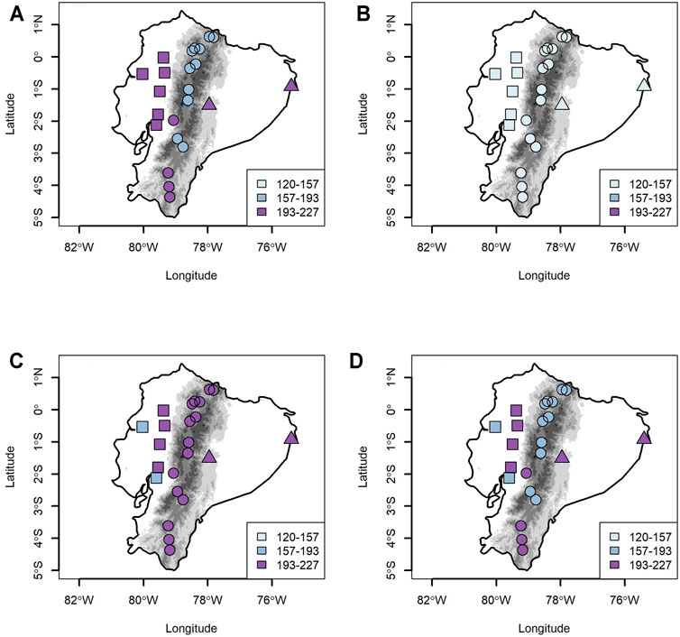
FIGURE 7. HRD mean value for the period 2041–2070 from CSIRO (A), GISS (B), and IPSL (C). Figure 7D is the ensemble that explains the median from three WGCMs.

HRD was calculated in every station for a year, and averages of all stations were plotted for every year (Figure 8). In Ecuador, the HRD index shows the number of days above P84Tmax from the base period. The CSIRO model displays a hard increase with peaks from −50 to +270 days (Figure 8A). The estimated number of days above P84Tmax for 2070 is approximately 250 days. In the period from 2011 to 2040 obtained from GISS, a high yearly variation of the HRD is observed, with peaks between −1 and 150 days. In addition, the trend displays a steep increase in the RCP 8.5 scenario, and for the period 2011–2040, a slight stabilization of the HRD is observed. Consequently, HRD exhibits growing increase, and for 2070, the HRD is between 150 and 170 days (Figure 8B). The HRD shows from IPSL model a high increase, specifically almost 150 warm days for 2011–2040, whereas a dramatic increase of 280 warm days is observed for 2070 (Figure 8C). The ensemble shows, in all temperature gauges, an increase in HRD between 20 and 100 days for 2011–2040 and in the period 2041–2070 peaks between 148 and 251 days (Figure 8D).

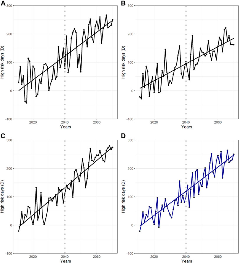
FIGURE 8. HRD of temperature gauges in Ecuador from CSIRO (A), GISS (B), and IPSL (C). (D) is the ensemble that explains the median from three WGCMs. Values of the HRD axis are between −100 and 300 days.

Analysis of High Risk Warming and High Risk Day Future Trends Under Representative Concentration Pathway 8.5

MKTM and SST were applied to all stations to analyze the trends of HRW and HRD for WGCM projections. Across the three regions of Ecuador, the probability of significance (p-value) was less than 0.05, and hence, the null hypothesis (Ho) was rejected (Tables 3, 4, and 5), thus, both indices showing a positive trend for future projections (Table 3).

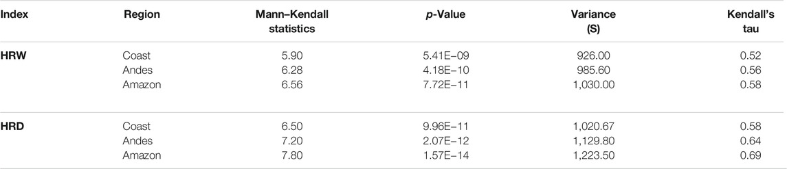
TABLE 3. Results of the Mann–Kendall model for the mean of the indices derived from the CSIRO model for all stations.

TABLE 4. Mann–Kendall model result of the mean of the all-station index in each region derived from the GISS model.

TABLE 5. Mann–Kendall model results of the mean of the all-station index in each region derived from the IPSL model.

Table 6 shows a small variation between the trends of the regions. Specifically, the HRW from the CSIRO model exhibits a decadal increase of 0.69° in the Coast, whereas in the Andes, SST is around 0.54°, and for the Amazon, the annual increase is 0.7°. The HRD shows an SST of 45.2, 40.0, and 45.9 days for the Coast, Andes, and Amazon, respectively. The SST from the CSIRO model displays the highest increase in the Amazon. The GISS model shows HRW values of 0.54°C, 0.52°C, and 0.57°C in the Coast, Andes, and Amazon, respectively; HRD values of 28.8 days in the Coast, 31.9 days in the Andes, and 30.4 days in the Amazon are also observed. The GISS model displays the highest values of warming indices in the Amazon. The IPSL model displays HRW values of 0.73°C in the Coast, 0.72°C in the Andes, and 0.91°C in the Amazon. The HRD index shows similar values in all regions, specifically SST values of 46 days in the Coast, 48 days in the Andes, and for 49 days in the Amazon.

TABLE 6. Mean of Sen’s estimated slope magnitude in each region for HRW and HRD, with a 95% confidence interval.

Discussion

The rise in global temperature has been accepted with high confidence (IPCC. et al., 2014, IPCC, 2021) as well as its impact on human health linked to excess morbidity and mortality mostly related to heat stroke (Ebi et al., 2020). The application of HRW and HRD indexes presented in this study provide direct and useful information for decision makers, public health professionals, and CC adaptation planners to assess the impact of CC on human health and to subsequently develop strategies to reduce such impacts (Christidis et al., 2019). Climate projections show a persistent increase in temperature under different scenarios of CC at global, regional, and local scales. For instance, the projections over China by 2050 displays an increase in the maximum temperature by 3.0°C–4.7°C under RCP 8.5 scenario (Wang et al., 2014). However, an increase of between 4.5°C and 5°C is expected over South America by the end of the century under RCP 8.5 (Riahi et al., 2011), similar incrasase is projected by Armenta et al. (2016) in RCP 8.5 by the end of the century over Ecuador.

The use of Qmap through PTF temperature correction exhibits good results over Ecuador showing a reduction in systematic bias, and the MAE and RMSE show good result correction as well. Also, Panjwani et al. (2021) found that in the case of India, the QUANR correction with trilinear transformation displays the best performance for temperature correction. Thus, Enayati et al. (2020) in Iran found that performance of the Qmap varied, depending on the transformation functions, parameters, and topographic conditions; also, PTF does not necessarily improve temperature projections. However, in Ecuador, Qmap methods do not show a relationship between topography and accuracy (Figure 3), while similar accuracy is observed applying the different Qmap methods in all regions (Table 2). Also, other more complex methods (e.g., Zhou et al. (2018); Crimp et al. (2019); Araya-Osses et al. (2020); Zhou et al. (2021)) could be analyzed in future studies in order to find a statistical downscaling method for each region (Coast, Andes, and Amazon) in Ecuador, which, because of its complex topography, may need a different correction method for each region. In addition, the extreme temperature values could be analyzed and how that influence in the bias correction in the future period.

The tendencies of HRW and HRD found by Christidis et al. (2019) for six continental regions of the world using the RCP 4.5 scenario project ranges between 0.237 and 0.209 for HRW and 2.787 to 6.518 for HRD. However, South America shows the highest values for HRD in the projections for 2,100, estimating a tendency of 6.518 days/decade, while the HRW shows an increase of 0.209 (K/decade) under the RCP 4.5 scenario. In our study of Ecuador, trends for both HRW and HRD using the RCP 8.5 scenario project higher values than for the RCP 4.5 scenario. The primary reasons for these higher values may be that 1) Christidis et al. (2019) used pre-industrial simulation data for the estimation of the 84th percentile of Tmax, while our baseline period was 1980–2005, and 2) the RCP 8.5 scenario projects a higher increase in temperature than RCP 4.5. The models have shown a consistent and strong increase in HRW and HRD over all Ecuador, although the models show some differences between the indexes. These results suggest that the population of Ecuador would face an increase in high mortality risk on the Coastal, Andes, and Amazonian regions in the following decades from 2040 to 2070. The deviation from the OT, increasing up to 5°C, and the increase in frequency of unsafe days, ranging from 100 to 250 days, would increase the number of deaths by heat stroke and mortal exacerbations of chronic diseases in people with preexisting conditions in Ecuador.

The World Health Organization (WHO) applied a similar approach to this study (Honda et al., 2014) to estimate the climate change-attributable heat-related excess number of deaths in different regions of the world, without adaptation actions to reduce the vulnerability of the population or mitigate the heat stress. It was estimated that tropical Latin America would have 1,808 excess number of deaths annually by 2030 and 5,912 by 2050 (WHO, 2014); however, these numbers only considered mortality, the impacts for morbidity, productivity loss, public health expenses, and indirect health care expenses, which can be very large (Silveira et al., 2019; Burkart et al., 2021). Thus, the results of the Ecuador HRW and HRD have several important applications, including to estimate mortality risk assessment to enhance health system emergency preparedness and response, and to develop public awareness and communication to individuals, authorities, and decision makers. As Ebi et al. (2020) states: “Limited understanding of the present impacts of climate change on public health restricts investment in building climate-resilient health systems.” Thus, the results of this study, provide a useful climate product that can be integrated into interdisciplinary studies for heat-health early warning systems and adaptation to climate change.

The need for an integrated and transformative approach embedded into climate change adaptation plans, knowledge of vulnerability, and risks of cities, mitigation measures, monitoring of extreme events, and public health awareness could help to prevent increase in mortality associated with heat warming (Ebi et al., 2020; Leal et al., 2018, 2019). The most impacted population would be the poorest, the vulnerable people, sensitive and with least adaptive capacity to respond and recover to the increased risk of heat on cities and peri urban areas (Leal et al., 2018; Litardo et al., 2021). Furthermore, analysis of duration and recurrence of warming events are important to reduce the mortality risk of Ecuadorian population.

Some limitations of this study are the length of the time series used in this analysis and the limited number of stations across the Ecuador territory, particularly in the Amazonian region. Finally, there is a need to validate those indices with mortality data for extreme events in the historical time series. Further research should explore modifications of the mortality risk indices presented in this study.

Conclusion

All the models project higher temperatures in the coastal and Amazon regions than in the Andes. The results of the WRF downscaling models show a positive bias; however, statistical downscaling reduces the bias and provides closer values to the temperature observed. The best correction method for Ecuador temperature is the quantile–quantile (PTF); however, other statistical downscaling methods could be applied to improve the temperature accuracy of the subregions, and its influence in extreme values could be analyzed.

The MKTM shows a positive tendency in all Ecuador, and the SST exhibits a steep increase trend of HRW and HRD. In addition, the Amazon region is projected to experience the highest increase in the HRW, while the HRD shows a similar increase in all the regions. Thus, the IPSL model shows higher spatiotemporal changes. An increase in warming events is projected for Ecuador by all models; the increase is consistent, and the temperature trends between models are similar for the regions. The rate of temperature increase is steep; by 2070, an increase of 3°C and 250 days above the 84th percentile of Tmax is projected.

The stronger increase in HRW and HRD in the medium term would be a climate change concern in Ecuador; human health impacts would be associated with excess deaths, and losses and damages caused by the heat stress and exacerbation of chronic diseases (Arjona et al., 2016). Although the increase in the near future may not be so great, in the long term (2070), the projections are very dramatic, showing a high slope of temperature in relation to historical conditions. Considering spatial-temporality of the HRW and HRD over all of Ecuador, climate conditions could come to play a crucial role in the habitability and sustainability of cities (Leal et al., 2019). The trend of indices in this study suggests a high risk of mortality that would affect the most vulnerable population in Ecuador. The primary limitations of this study are related to the need to evaluate the V-shape model for the climatic regions of Ecuador, and in addition, the mortality and health data would need to be included for an integrated climate–health assessment.

This study provides important climate service information for understanding the potential impact of CC in human health. Furthermore, temperature risk indices together with vulnerability analysis can be used to develop adaptation plan and strategies for human health in Ecuador.

Data Availability Statement

The meteorological data from ground stations used in this publication, is available through the INAMHI according to their data sharing policies, and the results of the Third National Communication through the Minister of Environment of Ecuador.

Author Contributions

LC, DU-F, MB-C, SS, LM, and MM conceptualized the study and developed the methodological design. MM analyzed the data and developed the script. LC, LM, DU-F, MB-C, SS, and MM prepared and revised the manuscript.

Funding

This publication is funded by the Escuela Superior Politecnica del Litoral (ESPOL), Guayaquil, and by the Escuela Politecnica Nacional (EPN) in Quito, Ecuador.

Conflict of Interest

The authors declare that the research was conducted in the absence of any commercial or financial relationships that could be construed as a potential conflict of interest.

Publisher’s Note

All claims expressed in this article are solely those of the authors and do not necessarily represent those of their affiliated organizations, or those of the publisher, the editors, and the reviewers. Any product that may be evaluated in this article, or claim that may be made by its manufacturer, is not guaranteed or endorsed by the publisher.

Acknowledgments

The authors thank INAMHI for providing ground stations\ data, to the Minister of Environment of Ecuador for sharing the downscaled results from the Third National Communication project, to the Red Ecuatoriana de Cambio Climatico (RECC) for the networking support in this project, and Bart Daly for early language editing of this paper.

References

Anderson, B. G., and Bell, M. L. (2009). Weather-Related Mortality. Epidemiology (Cambridge, Mass.) 20 (2), 205–213. doi:10.1097/EDE.0b013e318190ee08
Angus, J. E. (1994). The Probability Integral Transform and Related Results. SIAM Rev. 36 (4), 652–654. doi:10.1137/1036146
Araya-Osses, D., Casanueva, A., Román-Figueroa, C., Uribe, J. M., and Paneque, M. (2020). Climate Change Projections of Temperature and Precipitation in Chile Based on Statistical Downscaling. Clim. Dyn. 54 (9), 4309–4330. doi:10.1007/s00382-020-05231-4
Armenta, G., Villa, J., and Jácome, P. S. (2016). Proyecciones climáticas de precipitación y temperatura para Ecuador, bajo distintos escenarios de cambio climático. INAMHI (Instituto Nacional de Meteorología e Hidrología), 122. https://info.undp.org/docs/pdc/Documents/ECU/14%20Proyecciones%20de%20Clima%20Futuro%20para%20Ecuador%20en%20base%20a%20IPCC-AR5.pdf
Ballari, D., Giraldo, R., Campozano, L., and Samaniego, E. (2018). Spatial Functional Data Analysis for Regionalizing Precipitation Seasonality and Intensity in a Sparsely Monitored Region: Unveiling the Spatio-Temporal Dependencies of Precipitation in Ecuador. Int. J. Climatol 38 (8), 3337–3354. doi:10.1002/joc.5504
Bendix, J., and Lauer, W. (1992). Interpretation Rainy Seasons in ecuador and Their Climate-Dynamic Interpretation. Erdkunde, 118–134.
Boé, J., Terray, L., Habets, F., and Martin, E. (2007). Statistical and Dynamical Downscaling of the Seine basin Climate for Hydro-Meteorological Studies. Int. J. Climatol. 27 (12), 1643–1655. doi:10.1002/joc.1602
Burkart, K. G., Brauer, M., Aravkin, A. Y., Godwin, W. W., Hay, S. I., He, J., et al. (2021). Estimating the Cause-specific Relative Risks of Non-optimal Temperature on Daily Mortality: A Two-Part Modelling Approach Applied to the Global Burden of Disease Study. The Lancet 398 (10301), 685–697. doi:10.1016/S0140-6736(21)01700-1
Buytaert, W., Vuille, M., Dewulf, A., Urrutia, R., Karmalkar, A., and Célleri, R. (2010). Uncertainties in Climate Change Projections and Regional Downscaling in the Tropical Andes: Implications for Water Resources Management. Hydrol. Earth Syst. Sci. 14 (7), 1247–1258. doi:10.5194/hess-14-1247-2010
Campozano, L., Ballari, D., Montenegro, M., and Avilés, A. (2020). Future Meteorological Droughts in Ecuador: Decreasing Trends and Associated Spatio-Temporal Features Derived from CMIP5 Models. Front. Earth Sci. 8, 17. doi:10.3389/feart.2020.00017
Campozano, L., Célleri, R., Trachte, K., Bendix, J., and Samaniego, E. (2016). Rainfall and Cloud Dynamics in the Andes: A Southern Ecuador Case Study. Adv. Meteorology 2016, 1–15. doi:10.1155/2016/3192765
Chaturvedi, R. K., Joshi, J., Jayaraman, M., Bala, G., and Ravindranath, N. H. (2012). Multi-model Climate Change Projections for India under Representative Concentration Pathways. Curr. Sci. 103 (7), 791–802. http://www.jstor.org/stable/24088836
Chimborazo, O., and Vuille, M. (2021). Present-day Climate and Projected Future Temperature and Precipitation Changes in Ecuador. Theor. Appl. Climatology 143 (3), 1581–1597. doi:10.1007/s00704-020-03483-y
Christidis, N., Mitchell, D., and Stott, P. A. (2019). Anthropogenic Climate Change and Heat Effects on Health. Int. J. Climatol 39 (12), 4751–4768. doi:10.1002/joc.6104
Crimp, S., Jin, H., Kokic, P., Bakar, S., and Nicholls, N. (2019). Possible Future Changes in South East Australian Frost Frequency: An Inter-comparison of Statistical Downscaling Approaches. Clim. Dyn. 52 (1), 1247–1262. doi:10.1007/s00382-018-4188-1
Diaz Lozano Patino, E., and Siegel, J. A. (2018). Indoor Environmental Quality in Social Housing: A Literature Review. Building Environ. 131, 231–241. doi:10.1016/j.buildenv.2018.01.013
Ebi, K. L., Åström, C., Boyer, C. J., Harrington, L. J., Hess, J. J., Honda, Y., et al. (2020). Using Detection and Attribution to Quantify How Climate Change Is Affecting Health. Health Aff. 39 (12), 2168–2174. doi:10.1377/hlthaff.2020.01004
Enayati, M., Bozorg-Haddad, O., Bazrafshan, J., Hejabi, S., and Chu, X. (2020). Bias Correction Capabilities of Quantile Mapping Methods for Rainfall and Temperature Variables. J. Water Clim. Change 12 (2), 401–419. doi:10.2166/wcc.2020.261
Filho, W. L., Balogun, A. L., Olayide, O. E., Azeiteiro, U. M., Ayal, D. Y., Muñoz, P. D. C., et al. (2019). Assessing the Impacts of Climate Change in Cities and Their Adaptive Capacity: Towards Transformative Approaches to Climate Change Adaptation and Poverty Reduction in Urban Areas in a Set of Developing Countries. Sci. Total Environ. 692, 1175–1190. doi:10.1016/j.scitotenv.2019.07.227
Francou, B., Vuille, M., Favier, V., and Cáceres, B. (2004). New Evidence for an ENSO Impact on Low-Latitude Glaciers: Antizana 15, Andes of Ecuador, 0°28′ S. J. Geophys. Res. Atmospheres 109 (D18106), 17. doi:10.1029/2003JD004484
Goldberg, R. A., Tisnado M., G., and Scofield, R. A. (1987). Characteristics of Extreme Rainfall Events in Northwestern Peru during the 1982-1983 El Niño Period. J. Geophys. Res. 92 (C13), 14225–14241. doi:10.1029/JC092iC13p14225
Gudmundsson, L. (2012). Package ‘qmap.’. Methods 2012 (16), 3383–3390. doi:10.5194/hess-16-3383-2012
Gudmundsson, L. (2016). Statistical Transformations for post-processing Climate Model Output. Package qmap, 36. https://cran.r-project.org/web/packages/qmap/qmap.pdf
Gudmundsson, L., Bremnes, J. B., Haugen, J. E., and Engen-Skaugen, T. (2012). Technical Note: Downscaling RCM Precipitation to the Station Scale Using Statistical Transformations - a Comparison of Methods. Hydrol. Earth Syst. Sci. 16 (9), 3383–3390. doi:10.5194/hess-16-3383-2012
Haines, A., and Patz, J. A. (2004). Health Effects of Climate Change. JAMA 291 (1), 99–103. doi:10.1001/jama.291.1.99
Harari Arjona, R., Piñeiros, J., Ayabaca, M., and Harari Freire, F. (2016). Climate Change and Agricultural Workers' Health in Ecuador: Occupational Exposure to UV Radiation and Hot Environments. Ann. Ist Super Sanita 52 (3), 368–373. doi:10.4415/ANN_16_03_08
Heuzé, C., Heywood, K. J., Stevens, D. P., and Ridley, J. K. (2013). Southern Ocean Bottom Water Characteristics in CMIP5 Models. Geophys. Res. Lett. 40 (7), 1409–1414. doi:10.1002/grl.50287
Hibbard, K. A., Vuuren, Van, D. P., and Edmonds, J. (2011). A Primer on the Representative Concentration Pathways (RCPs) and the Coordination between the Climate and Integrated Assessment Modeling Communities. CLIVAR Exchanges 16 (2), 12–15. https://eprints.soton.ac.uk/194679/1/CLIVAR_Exchange_Special_Addition_No.56.pdf
Honda, Y., Kabuto, M., Ono, M., and Uchiyama, I. (2007). Determination of Optimum Daily Maximum Temperature Using Climate Data. Environ. Health Prev. Med. 12 (5), 209–216. doi:10.1265/ehpm.12.209
Honda, Y., Kondo, M., McGregor, G., Kim, H., Guo, Y.-L., Hijioka, Y., et al. (2014). Heat-related Mortality Risk Model for Climate Change Impact Projection. Environ. Health Prev. Med. 19 (1), 56–63. doi:10.1007/s12199-013-0354-6
IPCC (2021). “Summary for Policymakers,” in Climate Change 2021: The Physical Science Basis. Contribution of Working Group I to the Sixth Assessment Report of the Intergovernmental Panel on Climate Change. Editor V. Masson Delmotte, P. Zhai, A. Pirani, S. L. Connors, C. Péanet al. Cambridge University Press. In Press, 40.
Kovats, R. S., and Hajat, S. (2008). Heat Stress and Public Health: A Critical Review. Annu. Rev. Public Health 29 (1), 41–55. doi:10.1146/annurev.publhealth.29.020907.090843
Kyselý, J. (2004). Mortality and Displaced Mortality during Heat Waves in the Czech Republic. Int. J. Biometeorol. 49 (2), 91–97. doi:10.1007/s00484-004-0218-2
Leal Filho, W., Echevarria Icaza, L., Neht, A., Klavins, M., and Morgan, E. A. (2018). Coping with the Impacts of Urban Heat Islands. A Literature Based Study on Understanding Urban Heat Vulnerability and the Need for Resilience in Cities in a Global Climate Change Context. J. Clean. Prod. 171, 1140–1149. doi:10.1016/j.jclepro.2017.10.086
Limaye, V. S., Vargo, J., Harkey, M., Holloway, T., and Patz, J. A. (2018). Climate Change and Heat-Related Excess Mortality in the Eastern USA. EcoHealth 15 (3), 485–496. doi:10.1007/s10393-018-1363-0
Litardo, J., Palme, M., Borbor-Cordova, M., Caiza, R., Hidalgo-Leon, R., del Pilar Cornejo-Rodriguez, M., et al. (2021). Urban Heat Island Simulation and Monitoring in the Hot and Humid Climate Cities of Guayaquil and Durán, Ecuador. Springer Singapore: Advances in 21st Century Human Settlements. doi:10.1007/978-981-33-4050-3_7
Lockwood, J. (2009). “The Climate of the Earth,” in Atmospheric Science for Environmental Scientists. 2nd Edn, Editors C. Nick Hewitt, and A. V. Jackson (Hoboken, NJ, United States: Wiley-Blackwell), 20–23.
Mach, K. J., Mastrandrea, M. D., Bilir, T. E., and Field, C. B. (2016). Understanding and Responding to Danger from Climate Change: The Role of Key Risks in the IPCC AR5. Climatic Change 136 (3–4), 427–444. doi:10.1007/s10584-016-1645-x
Maraun, D., Wetterhall, F., Ireson, A. M., Chandler, R. E., Kendon, E. J., Widmann, M., et al. (2010). Precipitation Downscaling under Climate Change: Recent Developments to Bridge the gap between Dynamical Models and the End User. Rev. Geophys. 48 (3). doi:10.1029/2009rg000314
Matzarakis, A., Mayer, H., and Iziomon, M. G. (1999). Applications of a Universal thermal index: Physiological Equivalent Temperature. Int. J. Biometeorology 43 (2), 76–84. doi:10.1007/s004840050119
Modarres, R., de Paulo Rodrigues da Silva, V., and de, V. P. R. (2007). Rainfall Trends in Arid and Semi-arid Regions of Iran. J. Arid Environments 70 (2), 344–355. doi:10.1016/j.jaridenv.2006.12.024
Montero, J. C., Mirón, I. J., Criado-Álvarez, J. J., Linares, C., and Díaz, J. (2012). Influence of Local Factors in the Relationship between Mortality and Heat Waves: Castile-La Mancha (1975-2003). Sci. Total Environ. 414, 73–80. doi:10.1016/j.scitotenv.2011.10.009
Morán-Tejeda, E., Bazo, J., López-Moreno, J. I., Aguilar, E., Azorín-Molina, C., Sanchez-Lorenzo, A., et al. (2016). Climate Trends and Variability in Ecuador (1966-2011). Int. J. Climatol. 36 (11), 3839–3855. doi:10.1002/joc.4597
Morefield, P., Fann, N., Grambsch, A., Raich, W., and Weaver, C. (2018). Heat-related Health Impacts under Scenarios of Climate and Population Change. Int. J. Environ. Res. Public Health 15 (11), 2438. doi:10.3390/ijerph15112438
Moura, M. M., dos Santos, A. R., dos Santos, J. E. M., Alexandre, R. S., da Silva, S. F., de Andrade, M. S. S., et al. (2019). Relation of El Niño and La Niña Phenomena to Precipitation, Evapotranspiration and Temperature in the Amazon basin. Sci. Total Environ. 651, 1639–1651. doi:10.1016/j.scitotenv.2018.09.242
Navarro-Serrano, F., López-Moreno, J. I., Domínguez-Castro, F., Alonso-González, E., Azorin-Molina, C., El-Kenawy, A., et al. (2020). Maximum and Minimum Air Temperature Lapse Rates in the Andean Region of Ecuador and Peru. Int. J. Climatology 40 (14), 6150–6168. doi:10.1002/joc.6574
Ongoma, V., Chen, H., and Gao, C. (2018). Projected Changes in Mean Rainfall and Temperature over East Africa Based on CMIP5 Models. Int. J. Climatol 38 (3), 1375–1392. doi:10.1002/joc.5252
Panjwani, S., Naresh Kumar, S., and Ahuja, L. (2021). “Bias Correction of GCM Data Using Quantile Mapping Technique,” in Proceedings of International Conference on Communication and Computational Technologies. Editors S. D. Purohit, D. Singh Jat, R. C. Poonia, S. Kumar, and S. Hiranwal (Springer), 617–621. doi:10.1007/978-981-15-5077-5_55
Pasqui, M., and Di Giuseppe, E. (2019). Climate Change, Future Warming, and Adaptation in Europe. Anim. Front. 9 (1), 6–11. doi:10.1093/af/vfy036
Patz, J. A., Campbell-Lendrum, D., Holloway, T., and Foley, J. A. (2005). Impact of Regional Climate Change on Human Health. Nature 438 (7066), 310–317. doi:10.1038/nature04188
Piani, C., Haerter, J. O., and Coppola, E. (2010). Statistical Bias Correction for Daily Precipitation in Regional Climate Models over Europe. Theor. Appl. Climatology 99 (1), 187–192. doi:10.1007/s00704-009-0134-9
Riahi, K., Grübler, A., and Nakicenovic, N. (2007). Scenarios of Long-Term Socio-Economic and Environmental Development under Climate Stabilization. Technol. Forecast. Soc. Change 74 (7), 887–935. doi:10.1016/j.techfore.2006.05.026
Riahi, K., Rao, S., Krey, V., Cho, C., Chirkov, V., Fischer, G., et al. (2011). RCP 8.5-A Scenario of Comparatively High Greenhouse Gas Emissions. Climatic Change 109 (1), 33–57. doi:10.1007/s10584-011-0149-y
IPCCCore Writing Team (2014). Editors R. K. Pachauri, and L. A. Meyer. doi:10.1016/S0022-0248(00)00575-3Climate Change 2014: Synthesis Report. Contribution of Working Groups I, II and III to the Fifth Assessment Report of the Intergovernmental Panel on Climate Change]
Rusticucci, M., and Zazulie, N. (2021). Attribution and Projections of Temperature Extreme Trends in South America Based on CMIP5 Models. Ann. N.Y Acad. Sci. 1504 (1), 154–166. doi:10.1111/nyas.14591
Sa’adi, Z., Shiru, M. S., Shahid, S., and Ismail, T. (2020). Selection of General Circulation Models for the Projections of Spatio-Temporal Changes in Temperature of Borneo Island Based on CMIP5. Theor. Appl. Climatology 139 (1), 351–371. doi:10.1007/s00704-019-02948-z
Salmi, T., Määttä, A., Anttila, P., Ruoho-Airola, T., and Amnell, T. (2002). Detecting Trends of Annual Values of Atmospheric Pollutants by the Mann-Kendall Test and Sen’s Slope Estimates-The Excel Template Application MAKESENS. Helsinki, Finland: Finnish Meteorological Institute, 35.
Schwalm, C. R., Glendon, S., and Duffy, P. B. (2020). RCP8.5 Tracks Cumulative CO2emissions. Proc. Natl. Acad. Sci. USA 117 (33), 19656–19657. doi:10.1073/pnas.2007117117
Schweiker, M., Abdul-Zahra, A., André, M., Al-Atrash, F., Al-Khatri, H., Alprianti, R. R., et al. (2019). The Scales Project, a Cross-National Dataset on the Interpretation of thermal Perception Scales. Scientific Data 6 (1), 289. doi:10.1038/s41597-019-0272-6
Sen, P. K. (1968). Estimates of the Regression Coefficient Based on Kendall's Tau. J. Am. Stat. Assoc. 63 (324), 1379–1389. doi:10.1080/01621459.1968.10480934
Seneviratne, S. I., Donat, M. G., Mueller, B., and Alexander, L. V. (2014). No Pause in the Increase of Hot Temperature Extremes. Nat. Clim Change 4 (3), 161–163. doi:10.1038/nclimate2145
Sherwood, S. C., and Huber, M. (2010). An Adaptability Limit to Climate Change Due to Heat Stress. Proc. Natl. Acad. Sci. 107 (21), 9552–9555. doi:10.1073/pnas.0913352107
Shi, L., Kloog, I., Zanobetti, A., Liu, P., and Schwartz, J. D. (2015). Impacts of Temperature and its Variability on Mortality in New England. Nat. Clim Change 5 (11), 988–991. doi:10.1038/nclimate2704
Silveira, I. H., Oliveira, B. F. A., Cortes, T. R., and Junger, W. L. (2019). The Effect of Ambient Temperature on Cardiovascular Mortality in 27 Brazilian Cities. Sci. Total Environ. 691, 996–1004. doi:10.1016/j.scitotenv.2019.06.493
Song, J., Pan, R., Yi, W., Wei, Q., Qin, W., Song, S., et al. (2021). Ambient High Temperature Exposure and Global Disease Burden During 1990–2019: An Analysis of the Global Burden of Disease Study 2019. Sci. Total Environ. 787, 147540. doi:10.1016/j.scitotenv.2021.147540
Stekhoven, D. J., and Bühlmann, P. (2012). MissForest--non-parametric Missing Value Imputation for Mixed-type Data. Bioinformatics 28 (1), 112–118. doi:10.1093/bioinformatics/btr597
Stott, P. A., Christidis, N., Otto, F. E. L., Sun, Y., Vanderlinden, J. P., van Oldenborgh, G. J., et al. (2016). Attribution of Extreme Weather and Climate‐related Events. Wires Clim. Change 7 (1), 23–41. doi:10.1002/wcc.380
Tabari, H., Marofi, S., Aeini, A., Talaee, P. H., and Mohammadi, K. (2011). Trend Analysis of Reference Evapotranspiration in the Western Half of Iran. Agric. For. Meteorology 151 (2), 128–136. doi:10.1016/j.agrformet.2010.09.009
Vicente-Serrano, S. M., Aguilar, E., Martínez, R., Martín-Hernández, N., Azorin-Molina, C., Sanchez-Lorenzo, A., et al. (2017). The Complex Influence of ENSO on Droughts in Ecuador. Clim. Dyn. 48 (1–2), 405–427. doi:10.1007/s00382-016-3082-y
Vogel, R. M., and Kroll, C. N. (2000). Trends in Oods and Low Ows in the United States: Impact of Spatial Correlation. J. Hydrol. 240, 90–105. doi:10.1016/s0022-1694(00)00336-x
Vuille, M., Bradley, R. S., and Keimig, F. (2000). Climate Variability in the Andes of Ecuador and its Relation to Tropical Pacific and Atlantic Sea Surface Temperature Anomalies. J. Clim. 13 (14), 2520–2535. doi:10.1175/1520-0442(2000)013<2520:cvitao>2.0.co;2
Vuille, M., and Werner, M. (2005). Stable Isotopes in Precipitation Recording South American Summer Monsoon and ENSO Variability: Observations and Model Results. Clim. Dyn. 25 (4), 401–413. doi:10.1007/s00382-005-0049-9
Wang, L., Chen, W., and Zhou, W. (2014). Assessment of Future Drought in Southwest China Based on CMIP5 Multimodel Projections. Adv. Atmos. Sci. 31 (5), 1035–1050. doi:10.1007/s00376-014-3223-3
WHO. (2014). Quantitative Risk Assessment of the Effects of Climate Change on Selected Causes of Death, 2030s and 2050s.
Worfolk, J. B. (2000). Heat Waves: Their Impact on the Health of Elders. Geriatr. Nurs. 21 (2), 70–77. doi:10.1067/mgn.2000.107131
Yue, S., and Hashino, M. (2003). Temperature Trends in Japan: 1900–1996. Theor. Appl. Climatology 75 (1–2), 15–27. doi:10.1007/s00704-002-0717-1
Yunling, H., and Yiping, Z. (2005). Climate Change from 1960 to 2000 in the Lancang River Valley, China. Mountain Res. Develop. 25 (4), 341–348. doi:10.1659/0276-4741(2005)025[0341:ccftit]2.0.co;2
Zeng, Q., Li, G., Cui, Y., Jiang, G., and Pan, X. (2016). Estimating Temperature-Mortality Exposure-Response Relationships and Optimum Ambient Temperature at the Multi-City Level of China. Int. J. Environ. Res. Public Health 13 (3), 279. doi:10.3390/ijerph13030279
Zhou, X., Huang, G., Li, Y., Lin, Q., Yan, D., and He, X. (2021). Dynamical Downscaling of Temperature Variations over the Canadian Prairie Provinces under Climate Change. Remote Sensing 13 (21), 4350. doi:10.3390/rs13214350
Keywords: climate change, high risk warming, high risk days, climate extremes, increase of temperature
Citation: Montenegro M, Campozano L, Urdiales-Flores D, Maisincho L, Serrano-Vincenti S and Borbor-Cordova MJ (2022) Assessment of the Impact of Higher Temperatures Due to Climate Change on the Mortality Risk Indexes in Ecuador Until 2070. Front. Earth Sci. 9:794602. doi: 10.3389/feart.2021.794602
Received: 13 October 2021; Accepted: 13 December 2021;
Published: 31 January 2022.
Edited by:
Bin Yu, Environment and Climate Change, CanadaReviewed by:
Roger Rodrigues Torres, Federal University of Itajubá, BrazilXiong Zhou, Beijing Normal University, China
Copyright © 2022 Montenegro, Campozano, Urdiales-Flores, Maisincho, Serrano-Vincenti and Borbor-Cordova. This is an open-access article distributed under the terms of the Creative Commons Attribution License (CC BY). The use, distribution or reproduction in other forums is permitted, provided the original author(s) and the copyright owner(s) are credited and that the original publication in this journal is cited, in accordance with accepted academic practice. No use, distribution or reproduction is permitted which does not comply with these terms.
*Correspondence: M. J. Borbor-Cordova, meborbor@espol.edu.ec