Under-Ice Light Field in the Western Arctic Ocean During Late Summer

Introduction

The Arctic Ocean has been undergoing remarkable changes in the past decades. The most noticeable have been to the sea-ice cover (Stroeve and Notz, 2018; Meier et al., 2014; Comiso et al., 2008; Stroeve et al., 2012). Sea-ice extent has decreased in all seasons (Stroeve and Notz, 2018; Onarheim et al., 2018; Serreze et al., 2007, Stroeve et al., 2012), as well as its age and thickness (Lindsay and Schweiger, 2015; Maslanik et al., 1999; 2011; 2007; Renner et al., 2014). These changes have resulted in a shift of the sea-ice cover from thick, multi-year ice (MYI) to younger and thinner first-year ice (FYI) (Maslanik et al., 2011; 2007; Comiso, 2012). Additionally, observations show that the trend of snow depth, a major component in light transmission, has declined over recent years (Stroeve et al., 2020). The presence of melt ponds during late spring and summer also reduces the albedo of the ice and increases the amount of light transmitted to the water column (Perovich et al., 2002a; Light et al., 2008). The Chukchi and Beaufort seas are the parts of the Arctic Ocean at the forefront of this transition.

This transformation of the physical sea-ice environment, affects the partitioning of solar radiation passing through sea-ice. The result is a larger proportion of incoming solar radiation being able to reach the basal ice layer and upper ocean (Nicolaus et al., 2012). Increased transmission of solar radiation through sea-ice subsequently affects the heat and mass balance of the Arctic Ocean (Perovich et al., 2011; Nicolaus et al., 2012). Moreover, light is a crucial driver for sea-ice and ocean primary production (Mundy et al., 2009; Assmy et al., 2017). To study the growth of algae, and to understand how the sea-ice microbial community will adapt to a changing climate, it is essential to further advance in the field of radiative transfer through sea-ice (Pinkerton and Hayward, 2021). The absorption signature of ice algae on the spectral distribution of light under the ice, has been investigated during the last 3 decades (e.g., Legendre and Gosselin, 1991; Perovich, 1990; Mundy et al., 2007) and it has been used to develop algorithms to retrieve chlorophyll a (chl a) content in sea-ice, as proxy for biomass, based on under-ice light measurements. Normalised difference indices (NDI) have been used to retrieve chl a content in Antarctic pack ice in both summer (Melbourne-Thomas et al., 2015) and winter (Meiners et al., 2017), in Arctic pack ice (Lange et al., 2016), and in landfast sea-ice in both the Arctic (Mundy et al., 2007) and Antarctic (Wongpan et al., 2018). Recently, Castellani et al., 2020 used such algorithms to provide chl a estimates over large spatial scales derived (on the order of 10 km) with the same methodology in both the Arctic and the Antarctic.

Light transmission through Arctic sea-ice has been the subject of various studies through in situ observations, remote sensing, and modelling (e.g., Mundy et al., 2007; Light et al., 2008; Frey et al., 2011; Nicolaus et al., 2012; Katlein et al., 2019; Castellani et al., 2020; Stroeve et al., 2021; Pinkerton and Hayward 2021; Mundy et al., 2007; Light et al., 2008; Frey et al., 2011; Nicolaus et al., 2012; Katlein et al., 2019; Castellani et al., 2020; Stroeve et al., 2021; Pinkerton and Hayward, 2021). In situ optical measurements of under-ice light are performed using radiometers on static devices, as transect lines using remotely operated vehicles (ROV), or systems towed by ships (Lange et al., 2017; Massicotte et al., 2019; Castellani et al., 2020). These observations have been made in various regions across the Arctic Ocean, thus providing insight into the dynamics of the under-ice light field within different sea-ice regimes. However, it remains a challenge to conduct in situ field measurements of light transmission on a large scale in the Arctic due to logistical difficulties and financial constraints of sampling in high latitudes. Given that the characteristics of Arctic sea-ice are evolving, new observations, in present day, of sea-ice conditions are needed to constrain and improve parameterisations used for numerical models.

In this study, we discuss a set of sea-ice and snow measurements, under-ice light data, chl a and nutrient concentrations that were collected during two expeditions to the Chukchi Sea in August 2018 and August 2019, respectively. Late summer is a particularly interesting time to perform these measurements, as it represents a transition between the melting of the sea-ice and the autumn freeze-up. By late summer, the sea-ice and overlaying snow have undergone a series of melt-induced changes, including snow melt, the formation and subsequent drainage of melt ponds, reduction in bulk salinity, and the thinning of the sea-ice. These physical changes, coming from the surface, basal and lateral sea-ice melt processes, impact the light availability within and at the bottom of the sea-ice as well as in the water column. Quantifying how sea-ice melt will affect primary productivity within the sea-ice and water column remains a challenge (Gosselin et al., 1997; Lannuzel et al., 2020; Pinkerton et al., 2021).

The purpose of this study is to 1) better understand the differences in the light regime under ponded and unponded FYI and MYI, 2) provide evidence that will allow for better constraining of light attenuation parameterisations in numerical models, 3) to characterise the biological environment of late summer sea ice in the Chukchi Sea and 4) to provide the first NDI algorithm to retrieve in-ice chl a for this region and this season. The field campaigns and the measurements performed are described in sections The Arctic Cruises and Sea-Ice Stations, Light Measurements and Sea-Ice Properties, the spectral analysis tools employed are presented in Spectral Analysis followed by the Statistical Analysis and Normalised Difference Indices Algorithm sections Normalised Difference Indices Algorithm. The results of the analysis are presented in Results and discussed in Discussion.

Observations and Methodology

In order to better understand the physical and optical properties of sea-ice in the Chukchi Sea region in August, a number of ice floes were visited and different measurements were performed. The observations, their measurements protocols and the methodology followed to analyse them are described in the following sections.

The Arctic Cruises and Sea-Ice Stations

All measurements presented in this study were attained during two Arctic expeditions to the Chukchi Sea, by the South Korean ice breaking research vessel Araon, from August 4 to August 26, 2018 and from August 3 to August 27, 2019. During 2018, two FYI floes were visited, each with extensive melt ponds (Figures 1A–C; Table 1). The first ice floe (station IS 2018-1) was composed of a mixture of level and deformed FYI covered by a thin layer of wet snow. The ponds sampled consisted of freshwater, and were in a refrozen state, with an ice lid. The second ice floe (station IS2018-2) also consisted of refrozen ponded FYI, but the ice was clear of snow.

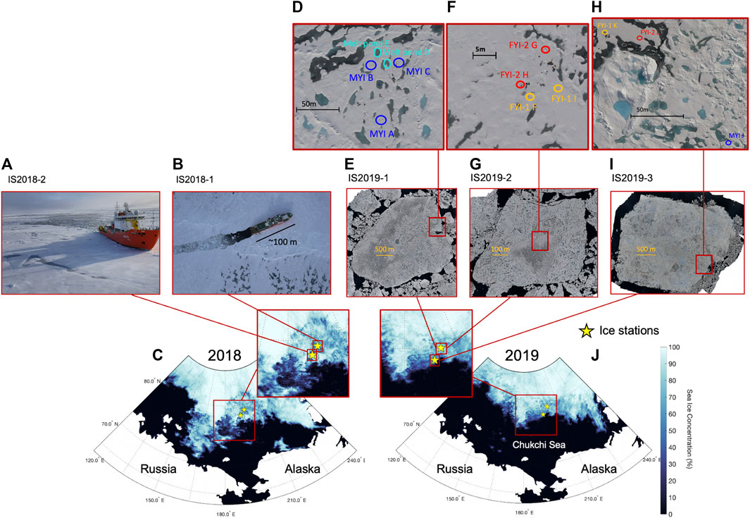
FIGURE 1. Maps of the sea-ice concentration (in %) at 3.125 km resolution in the Chukchi Sea region (C,J), locations of the sea-ice stations (A, B, C, E, G, I and J) and measurement sites (D, F and H). Sea-ice concentration was retrieved from daily Advanced Microwave Scanning Radiometer 2 (AMSR2) satellite data using the ARTIST sea-ice algorithm (ASI 5) from University of Bremen (Spreen et al., 2008), and averaged for the ice camps duration (18–21 August 2018 and 12–16 August 2019). Sea-ice stations are shown as stars on the sea-ice concentration maps and pictures of the floes and measurements sites are shown above the maps.

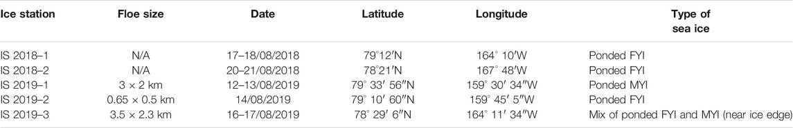
TABLE 1. Location of the ice floes visited during the ice camp and type of ice present at each location.

In 2019, more extensive measurements were performed on three different ice floes labelled IS2019-1, IS2019-2, and IS2019-3, respectively (Figures 1D–I). IS2019-1 was established on ponded MYI with a thin snow cover and the melt ponds sampled were freshwater ponds, with a newly formed ice lid. The second ice station (IS2019-2), was on a floe located 15 km in the south-west direction from IS2019-1, and consisted of level ponded FYI. As for IS2019-1, the snow cover was thin and wet. The last ice station (IS2019-3) was located near the edge of the ice pack and consisted of a mixture of level FYI and of deformed MYI, the latter covered by a thin layer of snow. In late summer, it can be particularly difficult to distinguish FYI from MYI using the salinity of the ice cores alone. Therefore, to accurately identify FYI from MYI, we use a suite of complementary information beyond salinity and temperature measurements of the ice cores. Our metrics include: 1) aerial photographic mosaics to identify different ice characteristics 2) in situ examination of surface features, such as the extent of weathering of ridges, as well as topographic evidence, such as undulating surface, which are tell-tale signs of MYI, and 3) the ice thickness and freeboard.

Light Measurements

During both years, under-ice hyperspectral measurements were performed using TriOS RAMSES Advanced Cosine Collector (SAMIP ACC-2) hyperspectral radiometers. The radiometers had an ultra-violet and visible coverage (from 190.8 to 735.2 nm) with a resolution of 2.2 nm in 2018, and a visible and near-infrared coverage (from 305.6 to 1,145.4 nm) with a resolution of 3.3 nm in 2019. The same type of sensor was used to measure incoming solar irradiance above the ice. Measurements of the incoming solar irradiance were performed coincidentally with the under-ice readings to ensure consistency. In all cases, the radiometers were levelled vertical and looking upward. In 2018, surface spectral albedo was collected for six different surface types of sea-ice. These were snow on sea-ice, bare-ice, open melt ponds, refreezing melt ponds, rough frozen melt ponds and smooth frozen melt ponds. Surface spectra were collected with an Analytical Spectral Devices–Field Spectrometer equipped with a remote cosine receptor to diffuse light. The instrument was set to report the average of 10 instrument measurements. On top of the instrument average, the reported value is the average ratio of three observational measurements of downwelling and upwelling solar radiation. Samples were collected at a minimum of 10 m apart.

During 2018, three sites were sampled on the first floe (IS2018-1, labelled 1–3), and two additional ones on the second floe (IS2018-2, labelled 4 and 5), for a total of 5 sites sampled. For each site, a 0.09 m diameter Kovacs core barrel was used to obtain the first core. The resultant hole was used to deploy the radiometer mounted on a “L arm” system (Wongpan et al., 2018). This system ensures that, under the ice, the radiometer is looking upright, and simultaneous X-Y tilt measurements guide the device to be level. The deployed radiometer was located at the end of the mechanical L arm, 1.05 m distance from the core hole. All measurements were performed at equal distance along a 180° circle arc, facing the direction of the Sun to avoid shadows. The sensor was as close as possible to the ice bottom and the surface of the ice in a range of 2 × 2 m, was kept pristine. All light measurements were performed six times per core before taking the average.

In 2019, a similar procedure to 2018 was followed with additional site manipulation experiments. These experiments were performed by conducting under-ice light measurements before and after removing the snow layer. The snow was removed by digging square shaped pits, with 0.50–1 m sides. These were dug at locations corresponding to the light measurements performed under the pristine surface. In total, 12 individual sites labelled from A to L, were visited across the three ice stations in which light transmission measurements were performed.

Sea-Ice Properties

The snow depth and grain size as well as ice thickness and freeboard were measured once per site. Snow depth was measured using a ruler during both campaigns and ice thickness and freeboard were measured at each core location using a measuring tape. In addition, during the 2019 campaign, the snow grain size was estimated using a 2 mm grid crystal card.

In order to deploy the L arm for under-ice light measurements, a hole was made by extracting an ice core. This core was used to measure the temperature and salinity profiles, as well as for nutrient sampling. Once extracted, the core was measured with a ruler and pictures were taken. The temperature of the ice was measured every 0.2 m using a wired digital thermometer probe (Traceable Digital Thermometer) and the core was cut in the field into 0.2 m sections from bottom, and placed in individual polyethylene bags. The ice cores were transported to the ship laboratory and melted without the addition of filtered sea water, in a dark room, at temperatures below 5°C. Once melted, the salinity was recorded for each ice core section using a calibrated portable conductivity meter (Thermo Scientific Orion Star A322) and nutrients concentrations (phosphate PO₄, nitrite and nitrate NO₂+NO₃, ammonium NH₄ and silicate SiO₂) were measured onboard using a four-channel continuous auto-analyser by applying standard colorimetric methods (QuAAtro; Seal Analytical). Note that the nutrients sampling for each site was performed only during 2019. For 2018, nutrients concentrations were obtained from other cores representative of the whole ice stations. Using the measured temperature and salinity profiles, we calculated the brine fraction profiles based on the relationship provided by Cox and Weeks (1983) and the coefficients for F₁(T) and F₂(T) for temperatures between −2 and 0°C from Leppäranta and Manninen (1988), when possible, by assuming the absence of air in the ice cores.

To obtain chl a concentrations, during 2018, two ice core were extracted at site 1 and site 5, one ice core at sites 2–4, and during 2019, three ice cores were extracted at each site. All cores extracted for chl a analysis were coinciding with under-ice light measurements. For analysis of chl a concentration, the ice cores were cut in the field in two parts: bottom and rest of the core. Since the measurements were conducted in late summer, when low concentration of biomass are expected, the bottom part was taken as 0.2 m to guarantee enough biomass for detection. Both parts were placed in separate polyethylene bags, transported to the ship laboratory and melted at <5°C, in the dark, with the addition of filtered sea water. The melted samples were filtered for chl a measurement using 0.7 μm glass fibre filters (GF/F; 24 mm; Whatman). Chl a concentrations were measured onboard using a calibrated Turner design Trilogy fluorometer, after extraction with 90% acetone (Parsons et al., 1984).

Spectral Analysis

Transmittance and Extinction Coefficients

In this study, we focus on the Photosynthetic Active Radiation (PAR) part of the spectrum (400–700 nm). The PAR range is also the biologically active part of the spectrum. To analyse the amount of light transmitted through sea-ice and snow, we compute the transmittance Tr (spectral and wavelength-integrated) following (Nicolaus et al., 2010) as:

where I_ui and I_ai (both in mW m⁻² nm⁻¹) are respectively the under-ice irradiance and above-ice incoming solar irradiance. Thereafter, we refer as Tr_snow and Tr_ice, for the transmittance through pristine surfaces and post snow removal, respectively.

The ice extinction coefficients were computed using post snow removal transmittances and by using an inverted formulation of the exponential decay as presented in Grenfell and Maykut (1977) as:

where κ_i is the ice extinction coefficient, h_i is the sea-ice thickness, h₀ is the surface scattering layer (SSL) thickness, Tr_ice is the wavelength-integrated measured transmittance, i_o is the bulk coefficient which parameterises the high extinction of incoming light which occurs at the surface and inside the SSL of sea ice (Grenfell and Maykut, 1977) and k_Bδz is the attenuation due to the presence of algal biomass in the sea-ice. The attenuation due to algae is given by k_Bδz with k_B = a’ $\times$ C, a’ equal to 0.02 m² (mg chl a⁻¹), C the chl a concentration, and δz the thickness increment (Castellani et al., 2017). While this computation of the ice extinction coefficients is based on a simpler model than the one developed in Light et al., 2008 and Ehn et al., 2008, it importantly gives us the opportunity to compare the results with large-scale models for which simple representations are widely used. Melt ponds in this study are covered with a newly formed refrozen lid, with no SSL, so their extinction coefficients are expressed as:

where ${\alpha }_i$ is the melt pond’s albedo, κ_w is the extinction coefficient, and h_w the depth of the pond water, respectively. As the water of the ponds was clear, we use κ_w = 0.14 m⁻¹. Using the light measurements performed under pristine surfaces, snow extinction coefficients are computed following:

where κ_s is the snow extinction coefficient, h_s the snow depth, ${\alpha }_s$ is the snow albedo and κ_i is the sea-ice extinction coefficient calculated using Eq. 3. Measurements without snow were not performed during 2018 thus, for the samples from this year, calculated ice extinction coefficients are only available for the melt ponds. Therefore, to compute the snow extinction coefficients for the 2018 unponded sites, we assume κ_i = 1 m⁻¹, the mean of the 0.5–1.5 m⁻¹ range presented by Grenfell and Maykut (1977). This value was also obtained by Lebrun (2019) based on under-ice irradiance observations performed in Baffin Bay during the GreenEdge campaign in 2015–1016.

Albedo and Extinction in the Surface Scattering Layer

During August 2018, albedo measurements were performed in parallel to the under-ice light measurements and covered different sea-ice surfaces (see Light Measurements). These measurements, obtained for overcast conditions, are used in Eqs 3, 4 to calculate the extinction coefficients for snow and for melt ponds. For the 2019 stations, there are no surface albedo measurements available. Instead, a single albedo value of 0.65 is chosen as representative of the conditions of the floes, e.g., ice covered by a thin layer of wet snow (Perovich et al., 2002a).

Following Grenfell and Maykut (1977), to calculate the ice extinction coefficient for unponded ice, we use the i_o parameter to account for the attenuation of light in the SSL. i_o represents the ratio of the downwelling irradiance at 0.1 m depth and at the surface, and the values used in our study depend on the physical characteristics of each site, on the weather conditions and on the state of the surface after snow removal. To assess the weather conditions (cloudy or clear sky) for the choice of the i_o value used in the calculation of the sea-ice extinction coefficients (see Transmittance and Extinction Coefficients), we use the ship’s 360-degree camera photographs of the sky obtained every 15 min. This methodology is different from the previous study from Katlein et al., 2019, where a fixed value of i_o was used. Furthermore, in Light et al. (2008, 2015) the ice was considered as a three-layer system consisting of the surface scattering and drained layers above the freeboard, and the interior of the ice below the freeboard. As our measurements were taken in late summer and the freeboard of the ice was below 0.1 m, the ice did not present a drained layer. Therefore, instead of using the “canonical” value of 0.1 m suggested by Maykut and Untersteiner (1971) for the SSL thickness, we consider the respective freeboard to be representative of the SSL thickness. In Supplementary Table S1, we show pictures of the pit surface and ice core for each point of measurement as well as the snow albedo and the associated i_o used to calculate the ice and snow extinction coefficient κ_i and κ_s. The i_o values used in the analysis are based on Grenfell and Maykut (1977) observations and are given in Supplementary Table S2.

Additionally, the layer of snow had a thickness of approximately 0.03 m, which is the canonical value for the snow SSL (Perovich, 2007). Based on this, we assume that the calculated κ_s represents the extinction of light in snow happening in the SSL. Therefore, the use of the constant i_o to parameterise the extinction in the snow is not needed.

Normalised Difference Indices Algorithm

A comparison between coincidence measurements of under-ice irradiance and chl a concentrations is used to develop an NDI algorithm (Mundy et al., 2007) for the Chukchi Sea in August. Values of integrated chl a lower than 0.1 mg m⁻² are excluded from the analysis (Castellani et al., 2020) which results in a total of 18 coincident measurements of under-ice irradiance and integrated chl a used to develop the NDI algorithm. Spectra are interpolated at 1 nm wavelength resolution and the NDI is calculated for all possible wavelength combinations in the PAR range according to:

where I_ui is the under-ice irradiance and λ₁ and λ₂ are for the wavelength pairing. Minimum distance between wavelengths is set as 5 nm. The NDI for each wavelength pair are correlated with the integrated chl a values and the resultant Pearson correlation coefficients are placed in a matrix to select the most significant wavelength pair. We then use a linear model to explore the relationship between predicted chl a from the NDI algorithm and integrated chl a from the ice cores.

Statistical Analysis

In order to statistically differentiate the light transmission through a range of MYI and FYI types, a statistical analysis is performed using the statistical functions from Python’s SciPy package (version 1.2.1). We verify the normality of the transmittance measurements and extinction coefficients for each ice group, by using the Shapiro-Wilk test (Shapiro and Wilk, 1965). This test is used to evaluate how likely the data was drawn from a Gaussian distribution. When a comparison between groups is performed in this study, we use the two-samples independent Students’s t-test to assess whether the two groups are significantly different with a significance level of 0.05.

Results

The measurements and subsequent analysis are described in the following sub-sections from snow and sea-ice physical properties, to their optical properties and characterisation of the biological state of the sea-ice during the two cruises.

Sea-Ice Thickness, Physical Properties and Snow Cover

The FYI (both ponded and unponded) sampled on IS2018-1 (Figure 1B) had a thickness ranging between 0.7 and 1.25 m. The snow cover when present was wet and melting with depths of approximately 0.03 m. On IS2018-2 (Figure 1A), the FYI thickness ranged between 0.40 and 0.88 m with similar snow conditions as the first floe (IS2018-1). The two melt ponds sampled (each on a different ice floe) were 0.58 and 0.30 m deep, overlying a sea ice of 0.40 and 0.60 m thickness, respectively and both had a refrozen lid of ∼0.1 m. The salinity profiles (Figure 2A, left panel, purple lines) from the ice cores extracted at the unponded FYI sites show an increasing salinity with depth, ranging from a minimum of 0.4 at the surface to a maximum of 2.3 at the bottom of the core. For the ponded FYI, this range extended from 0.4 at the surface to 1.7 at the bottom of the core. As for the temperature profiles (Figure 2A, middle panel), overall, they show a slight decrease with depth; with surface temperatures around −1°C and bottom temperatures just lower than −2°C. For ponded and unponded FYI sites, the brine fraction profiles are constants with depth with the volume of brine remaining below the threshold of permeability of 5%. Note that during the 2018 campaign, no detailed visual inspection of the ice cores was performed.

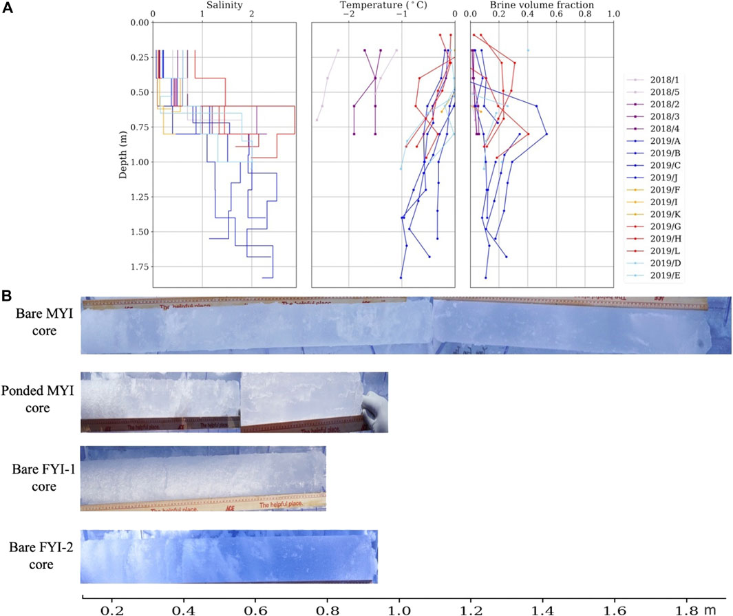
FIGURE 2. Physical properties and typical core pictures of sea ice for all sites. (A) Salinity, temperature (°C), and brine volume fraction profiles for the 2018 and 2019 sea-ice sites as a function of depth (m) in purple (2018 unponded and ponded FYI), blue (2019 unponded and ponded MYI), orange (FYI-1) and red (FYI-2). (B) Typical core pictures collected for unponded and ponded MYI, unponded FYI-1 and FYI-2, respectively.

The sites on IS2019-1 were MYI with a sea-ice thickness ranging between 0.78 and 1.70 m. The snow was melting and had a depth between 0.03 and 0.04 m. The snow grain size was approximately 0.5 mm. Sites on IS2019-2 were FYI with a thickness ranging from 0.77 to 0.92 m and the snow cover was very similar to the one found on IS2019-1. Finally, on IS2019-3, which was near the ice edge, the sea-ice thickness of the MYI ranged between 1.50 and 1.60 m while the FYI thickness ranged between 0.63 and 1.17 m. For all sites and floes, between the snow and the sea-ice surface, a loose granular layer, part of the sea ice, was present and made up of larger, transparent crystals that were generally embedded to the sea-ice surface. This layer forms part of SSL on top of the sea ice. In fact, as for our measurements, the SSL is often found to have a very granular structure (Grenfell and Maykut, 1977; Light et al., 2008).

Based on a comprehensive analysis of the sea-ice thickness, physical properties and core pictures, we are able to identify four different groups among the sea-ice sites sampled during 2019.

The first group consist of all the MYI samples (sites A, B, C and J, Table 2), for which the ice cores are made mostly of columnar ice (Figure 2B, upper core), with the thickness of the SSL ranging between 0.03 and 0.1 m. The salinity profiles (Figure 2A, left panel, blue lines) are fresh and show an increase in salinity with depth from below 0.025 to ∼2.5 followed by a decrease at the bottom resulting in an inverted C-shape. The temperature of the MYI cores decreases with depth from ∼0°C at the surface to between −0.35 and −1°C at the bottom of the cores. For the brine fraction (for which we assumed that no air was present), for most MYI sites, it is above the volume threshold of 5% above which, sea ice becomes permeable (Golden et al., 1998) but below 40% brine fraction (Figure 2A, right panel), without a strong increase near the middle of the core. One site displays a brine fraction near ∼53% between 0.6 and 0.8 m depth before decreasing towards the bottom (<25%).

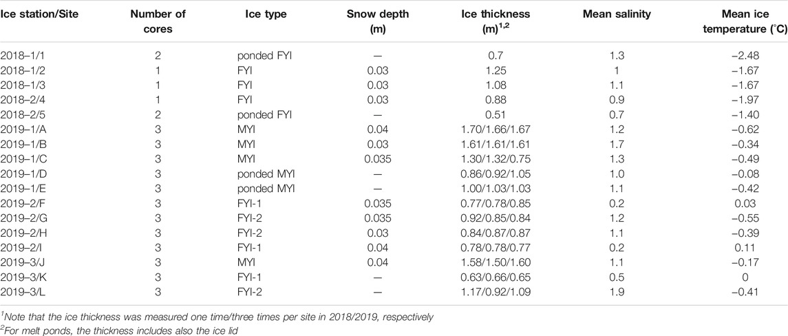
TABLE 2. Sites visited at each ice station in both years with, for each site: number of light measurements taken, sea-ice condition and groups (MYI, FYI-1, FYI-2, and melt ponds), snow depth (m), ice thickness (m), calculated average ice salinity (measurements with a conductivity meter Thermo Scientific Orion Star A322) and average ice temperature (°C).

Based on the characteristics of the FYI samples, they can be split into two groups: FYI-1 and FYI-2. FYI-1 sites (sites F, I, and K, Figures 1F–H and Table 2) have a thickness ranging between 0.63 and 0.85 m and the ice cores’ structure consists of large pores and channels (Figure 2B) saturated with meltwater. As the freeboard measured 0.01–0.02 m, the SSL was considered as thin but present. For two of the three FYI-1 sites, the vertical salinity profiles (Figure 2A) show an increasing salinity with depth from ∼0.1 at the surface to ∼0.4 at the bottom. Furthermore, the temperature profiles (Figure 2A, middle panel, orange lines) show temperatures near 0°C which points to an advanced stage of melt. Due to the strong level of decay, the extracted ice was particularly porous, suggesting a high air volume (after extraction) and a large loss of brines. Sea-ice density was not measured in this study, and thus, the volume of air present is unknown which prevents us from calculating brine volume fraction for this group. We consider that this group represents FYI that has undergone extreme melt and displays low structural integrity (decayed ice).

FYI-2 (sites G, H, and L, Figures 1F–H and Table 2) cores, have a sea-ice thickness ranging between 0.84 and 1.17 m. In this group, the ice cores consist of a different structure than that of FYI-1. They are composed of a SSL of 0.03–0.04 m and clear, columnar ice for the rest of the core. The salinity profiles show an increasing salinity with depth from 0.1–0.8 to 1.9–2.9 (Figure 2A, red lines) and a slight decrease towards the bottom. Temperatures mostly decrease with depth from ∼0°C to between −0.5 and −1°C. Brine volume fraction increases from the surface until approximately the middle of the cores with a maximum of ∼40% and decreases towards the bottom of the cores.

The last group corresponds to ponded MYI (sites D and E, Figure 1D and Table 2). Sea-ice thickness under the melt ponds ranges between 0.78 and 1 m, and the depth of meltwater within each pond is between 0.28 and 0.40 m, with a refrozen lid of 0.03–0.08 m. The water of the two ponds has a salinity of 0.78 and 0.53, respectively. The sea-ice temperature and salinity below the meltwater (Figure 2A, left and middle panels) respectively decreases and increases with depth; with temperatures near 0°C at the surface, reaching around -1°C at the sea ice/ocean interface and salinities close to 0.5 at the surface and reaching 2 at the bottom interface.

Optical Properties

Transmittance

We analyse the spectral transmittance as a function of wavelength for 1) the pristine snow-covered ice (and refrozen melt ponds) and 2) snow-free ice (where snow was removed) over all groups (Figure 4). Note that for the MYI measurements the weather was cloudy with high-altitude clouds which cleared before ponded MYI measurements and the visibility was high. The weather conditions for the FYI measurements were clear with very little high-altitude clouds.

Spectrally resolved transmittance varies between ice types. For both MYI and FYI-2, the transmittance is almost constant up to 500 nm and then decreases to 0 for wavelengths above 700 nm, in both pristine and snow-free cases. Similarly, FYI-1 decreases from 400 to 700 nm, but instead of falling towards ∼0 as for MYI and FYI-2, the spectral transmittance remains at a low level of ∼0.1 between 750 and 850 nm. Melt ponds show a marked increase from 300 nm with a peak at 400 nm and then similarly decrease to 700 nm. For the snow-free MYI (Figure 3A), the peak transmittance ranges between 0.06 and 0.09 (∼380 nm) while for ponded MYI (Figure 3B), the peak transmittance ranges from 0.3 to 0.4. The average peak transmittance is 0.21 and 0.11 for respectively, FYI-1 and FYI-2 (Figures 3D,E). The effect of a snow-cover, though in our case only a few centimetres thin, is also noticeable for all wavelengths, but stronger in the range 300–600 nm (Figures 3A,D,E). As expected, melt ponds, on both FYI and MYI, result in larger transmittances due to much thinner sea ice and the presence of melt water (Nicolaus et al., 2012), with large similarities between the two. The above- and under-ice (average and standard deviation) spectral irradiance for all sites (Supplementary Figure S1) illustrate similar features as the transmittance with a lower under-ice average peak transmittance of 55 mW m⁻² s⁻¹ for FYI-2 compared to the average peak transmittance of 101 mW m⁻² s⁻¹ for FYI-1 with a similar above-ice solar incoming irradiance (peak of ∼530 mW m⁻² s⁻¹ at 479 nm). The mean and standard deviation values of wavelength-integrated transmittances when snow is removed (Figure 4A and Table 3) also highlight differences between sea-ice types with 0.154 ± 0.039 (N = 9) for FYI-1, 0.086 ± 0.017 (N = 9) for FYI-2, 0.048 ± 0.011 (N = 12) for the MYI and 0.241 ± 0.038 (N = 6) for the MYI melt ponds. In comparison, the transmittances through pristine surfaces (Figure 4B) remain mostly below 0.05 for MYI, and around 0.05 for FYI-1 and -2 with the exception of the two sites that were not covered by snow (site K and L on IS2019-3, Figure 1H).

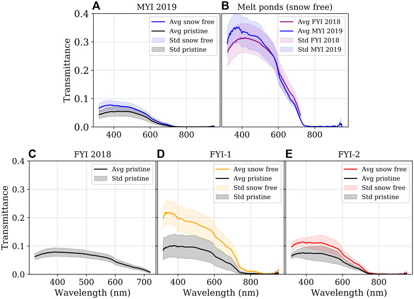
FIGURE 3. Spectral transmittance for different ice conditions: snow covered ice, snow-free ice and ponded ice, in both 2018 and 2019. For each category, the data are combined alongside the average and standard deviation. (A) MYI, with snow (grey) and snow-free (blue). (B) Melt ponds (MP), for FYI 2018 (purple) and MYI 2019 (blue). (C) FYI from 2018, with snow (grey). (D) FYI group 1 (FYI-1), with snow (grey) and snow-free (orange). (E) FYI group 2 (FYI-2), with snow (grey) and snow-free (red).

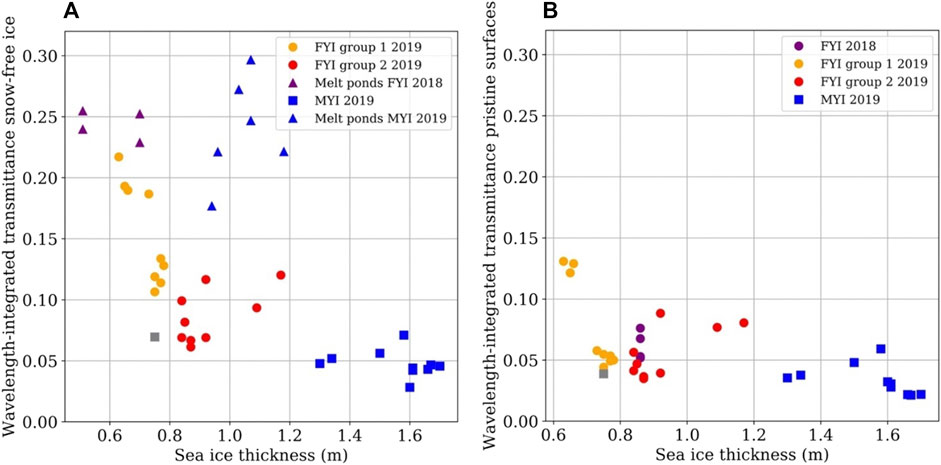
FIGURE 4. Wavelength-integrated transmittance through snow-free sea ice (A) and pristine surfaces (B) as function of sea-ice thickness. MYI cores are in blue squares, FYI from 2018 in purple circles, FYI-1 cores in orange circles, FYI-2 cores in red circles and melt pond cores in purple triangles (FYI/2018) and blue triangles (MYI/2019). The grey square corresponds to core C3, and was not considered during the analysis as it was too close to a melt pond.

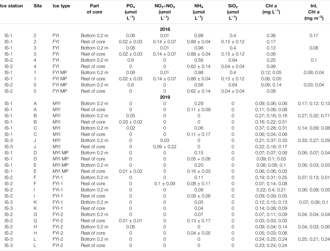
TABLE 3. Nutrients and chl a concentrations sampled for each site. The sites have been sorted according to the year and group. For the chl a, an integrated value is also given for each core. “0” means a neglibible concentration or below the detection limit.

Extinction Coefficients

The range of ice extinction coefficients varies for each group (Figure 5). For FYI-1, κ_i ranges between 1.10 and 1.93 m⁻¹ (1.49 ± 0.28 m⁻¹ (N = 9), Figure 5A) while for FYI-2, κ_i ranges between 0.73 and 1.33 m⁻¹ (1.12 ± 0.19 m⁻¹ (N = 9), Figure 5B). MYI cores display a large range of κ_i between 0.59 and 1.58 m⁻¹ (1.24 ± 0.26 m⁻¹ (N = 12), Figure 5C) as well as melt ponds with κ_i varying from 0.66 to 1.30 m⁻¹ (0.91 ± 0.21 m⁻¹ (N = 6), Figure 5D) for MYI ponds and between 1.44 and 2.24 m⁻¹, with an average of 1.84 m⁻¹ (N = 4), for FYI ponds. Data from 2019 core 3 at site C is excluded from this analysis because the core was situated very close to a melt pond (within 2 m), and thus the light coming through the melt pond contaminated the readings. Data from core 1 at site H shows a very small extinction coefficient but is not excluded from the analysis. The pictures of the ice cores (Figures 5E–H) are shown alongside the extinction coefficient’s sub-figures and allow to associate each group with the according typical core from the group. The average ice extinction coefficients for the decayed FYI-1 are higher than both the average ice extinction coefficients for FYI-2 and MYI (see Table 4). The values derived for the sea-ice extinction coefficients are also a function of the i_o values, and of the SSL thickness. These are individually selected for each site according to the freeboard, the inspection of the surface of the pit and the top layer of each ice core (see Supplementary Table S1 and Albedo and Extinction in the Surface Scattering Layer). Student’s t-tests (Table 5) show that FYI-1 and FYI-2 average ice extinction coefficients are significantly different with a p-value of 0.006, while the difference is not significant between FYI-1 and the MYI group as well as between FYI-2 and the MYI group with p-values > 0.05.

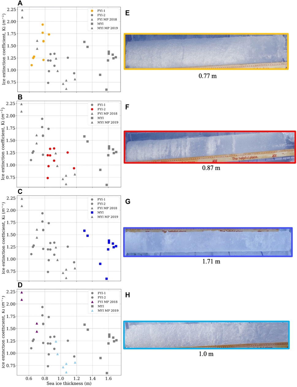
FIGURE 5. Sea-ice extinction coefficients as function of the sea-ice thickness. (A) FYI-1 in orange. (B) FYI-2 in red. (C) MYI in blue. (D) Melt ponds (MP) in purple (FYI) and light blue (MYI). Representative pictures of the ice cores for each group are displayed as (E) FYI-1, (F) FYI-2, (G) MYI and (H) MYI MP.

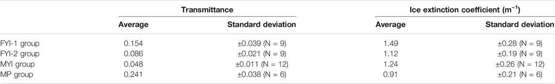
TABLE 4. Average and standard deviation for the transmittance and the ice extinction coefficient (in m⁻¹) for each group. The number of measurements is given as (N = X).

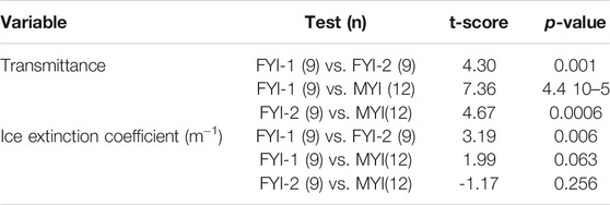
TABLE 5. Results of the Student’s t-tests (t-score, p-value) performed between the different groups (FYI-1, FYI-2, and MYI) for transmittance and ice extinction coefficients.

The snow extinction coefficients ${\kappa }_s$ (Figures 6A,B), for FYI in 2018, vary from 18 to 37.1 m⁻¹. For 2019, snow extinction coefficients vary from 2.7 to 13.5 m⁻¹ for MYI, from 13.4 to 22.3 m⁻¹ for FYI-1, and from 22.9 to 30.1 m⁻¹ for FYI-2. We note that the numbers of snow measurements are reduced, preventing us from calculating averages. It is also interesting to note that the snow cover is rather thin and uniform (from 0.03 to 0.04 m), contrasting with the high variability encountered in the calculated snow extinction coefficients (Figure 6A). The snow grain size varies from 0.5 to 1.4 mm (Figure 6B). While the smallest and biggest grains are coincident with MYI sites, intermediate values of 0.8 and 1.0 mm are found for FYI sites.

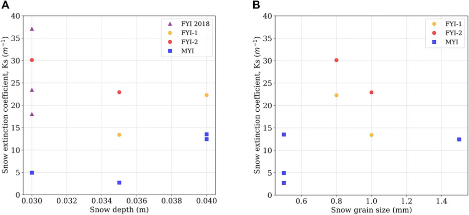
FIGURE 6. Snow extinction coefficients as a function of the snow depth (A) and the snow grain size (B). FYI sites in 2018 are represented with a purple triangle, FYI group 1 and FYI group 2 in orange and red respectively with a circle and MYI sites with a blue square.

Chl a Concentration and Nutrients

Chl a concentrations for the bottom 0.2 m of the ice cores vary from 0.06 to 0.37 mg m⁻³ for MYI cores, from 0.05 to 0.14 mg m⁻³ for melt ponds on FYI and MYI, from 0.12 to 0.4 mg m⁻³ for FYI-1 and from 0.04 to 0.25 mg m⁻³ for FYI-2 (Figures 7A,B). The chl a concentrations in the rest of the cores are lower for FYI-1 (from 0.05 to 0.14 mg m⁻³) and FYI-2 (from 0.03 to 0.06 mg m⁻³), with the exception of site L (FYI-2, IS2019-3, Figure 1H), for which the rest of the core concentrations are about the same as in the bottom 0.2 m (0.23–0.24 mg m⁻³). For some cores within MYI, concentrations are higher in the upper part of the core compared with the bottom (Figure 7B; Table 3). Average integrated chl a concentrations (Figure 8A and Table 3) for FYI-1 and FYI-2 are 0.08 and 0.11 mg m⁻² respectively, the last being similar to the average concentration of 0.12 mg m⁻² from the 2018 FYI. For FYI-1, the integrated chl a concentrations slightly decrease with the increasing under-ice irradiance. The average concentration is higher for MYI (0.24 mg m⁻², Figure 8A) without an effect on the under-ice irradiance and lower for the melt ponds (0.048 mg m⁻², Figure 8B) for both FYI in 2018 and MYI in 2019. The light attenuation factors due to the chl a (k_Bδz, see Sea-Ice Properties) are similar for all the sites and vary from 0.993 (MYI) to 0.998 (FYI-1 and melt pond sites).

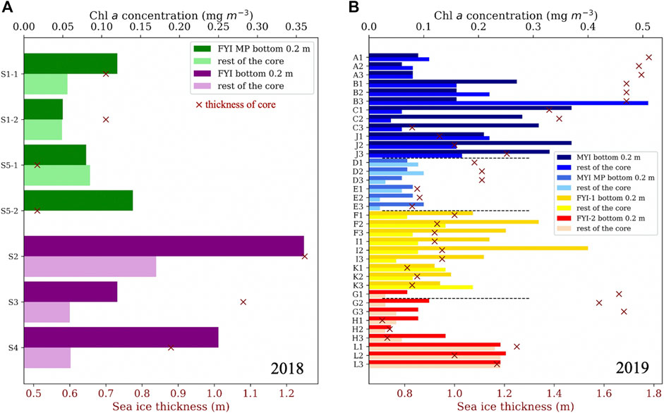
FIGURE 7. Chl a concentration (mg m⁻³) for the bottom 0.2 m (dark colour) and the rest of the core (light colour) for: (A) sites in 2018, and (B) sites in 2019. The colours separate the different ice conditions: blue for MYI, green and lighter blue for the MPs (FYI in 2018 and MYI in 2019), purple for FYI in 2018, yellow for FYI-1 and red for FYI-2. The crosses in both panels represents the ice core thickness (m). Note: there is no chl a concentration for the rest of the second core of site 5 in 2018 due to part of the core being lost during coring.

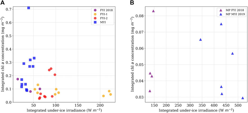
FIGURE 8. Integrated chl a concentration over the whole ice column for each site for (A) unponded ice and (B) melt ponds, as a function of the wavelength-integrated irradiance for unaltered sites. Note the different under-ice irradiance (x-axis) and chl a concentration (y-axis) limits for the melt ponds in (b).

For the NDI algorithm, the correlation matrix results in the highest correlation being near the second chl a absorption peak (∼670 nm) for the wavelengths 665 and 670 nm (Figure 9A), thus resulting in the predicted chl a being calculated as:

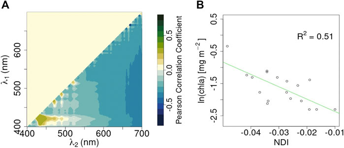
FIGURE 9. NDI’s correlation matrix for the all wavelength pairs (A) and predicted chl a concentration as a function of the NDI (B).

The comparison between predicted and measured chl a shows that NDI wavelength pairs (Figure 9A) explain only 51% (Figure 9B) of the total variability (R² = 0.51) in algal biomass. This is mainly due to the high heterogeneity of the surface of summer sea-ice that has undergone several melting and refreezing events, and to the very low biomass present. Previous studies have shown that also snow correlates with wavelengths close to the second algal absorption peak (e.g., Mundy et al., 2007; Wongpan et al., 2018; Mundy et al., 2007; Wongpan et al., 2018). However, in the present case we can exclude the effect of snow because of the advanced stage of melting of the surface and because the thin snow layer present was very uniform between the sampling sites (Lange et al., 2016). However, these measurements still include the effect of the snow surrounding the snow-free sites.

For IS2018-1, small concentrations of all nutrients are found in the bottom 0.2 m of the cores with 0.06, 0.01, 0.98 and 0.4 μmol L⁻¹ of phosphate, nitrite + nitrate, ammonium and silicate, respectively (Table 3). In the rest of the cores, concentrations are also small, never exceeding 1 μmol L⁻¹ compared to values on average above 20 mmol m⁻² reported by Yun et al., 2016 during spring and summer for the Northern Chukchi Sea. For IS2018-2, nitrite + nitrate concentrations are negligible for the whole core and below 0.65 μmol L⁻¹ for other nutrients. For the 2019 campaign, overall, values of nutrients are often below detection limit. This is true especially for silicate and nitrite + nitrate. Ammonium is present in small concentrations in the bottom of the ice cores with a maximum of 0.3, 0.2, 0.2 and 0.07 μmol L⁻¹ for MYI, ponded MYI, FYI-1 and FYI-2 respectively. No phosphate is found in FYI-1 while small concentrations (below 0.1 μmol L⁻¹) are measured in FYI-2 and MYI especially in the top of the cores.

Discussion

In this section, we discuss the results of our study, compare our data with data from previous studies and open the discussion for the future of Arctic sea-ice in the Chukchi Sea region.

Physical Properties and Sea-Ice Conditions

The thickness of the sea-ice types we encountered fall within the range of previously observed thicknesses of 0.1–2.45 m (average of 0.95 m) for this season and region such as reported by Wang et al., 2021 during multiple cruises in the Chukchi Sea performed in August between 2008 and 2016. Arrigo et al., 2012 reported increasing sea-ice thickness values in early summer 2010–2011 in the Chukchi Sea from 0.77 m near the ice edge, to an average of 1.21 m 120 km away from the ice edge, in agreement with our measurements. While Wang et al., 2021 documented sea ice that was a mix of MYI and FYI, they did not report any decayed sea ice of the kind we came across. Frantz et al., 2019, on the other hand, report rotten sea ice found during July, at a lower latitude of 71.29°N, on their survey of shore-fast ice near Barrow, Alaska. The late stage of sea-ice decay they describe in their study is very similar to the state of the FYI-1 type we encountered with temperatures of the ice near 0°C along the whole profile and salinities lower than 2. Compared to the earlier study of Melnikov et al., 2002, at similar latitudes of 75°–80°N and longitudes of 165°E to 150°E, but later in the season, the ice we sampled was warmer and less saline, pointing to a further evolved seasonal melting stage than in the past. The low salinity found in group FYI-1 is likely due to the advanced state of melting through numerous previous flushing events, with high desalinization during the brine release process. As the ice from FYI-2 cores was sampled in sites located 2–30 m from FYI-1 sites, we have to assume that ambient melting conditions for FYI-1 and FYI-2 were similar. The physical characteristics from FYI-1 suggest that the permeability is higher than for FYI-2, leading to a more porous and thus weaker internal structure. This points to the importance of the history of the ice, as ice forming in very cold conditions (e.g., leads opening in winter) might result in less brines released in the water, leading to larger, in number and size, brine pockets that might render the ice more porous. We suggest that its properties and overall lower integrity, decrease the potential survival of FYI-1 for the rest of the melting season compared to FYI-2.

Optical Properties

Light Transmission Through Sea ice and Snow

Both FYI groups show a larger range of transmittances and higher transmittance values compared to the MYI group. Average transmittance values for snow-free FYI-1 and FYI-2 are different by almost a factor of two (0.154 and 0.086) and the MYI group has an average snow-free transmittance almost two times smaller (0.048) than FYI-2. Student’s T-tests performed between groups show that their transmittances are all significantly different with p-values lower or equal to 0.001 (Table 5). The differences between groups are reduced when the transmittance is measured with snow being present (Figure 4B), which highlights the crucial role of snow in the transmission of light through sea-ice. For FYI-1 ice cores, we document a light transmission approaching that of the melt ponds. This indicates that, if more of the FYI would attain the state of decay of FYI-1 during late summer, a higher amount of light may be capable of reaching the interior of the ice and the upper-ocean. The melt pond group has average transmittances five times higher than for unponded MYI, a consequence of the structure (sea ice, meltwater and ice lid) of the melt ponds observed in this study. The average transmittances through ponded FYI in 2018 are the same as through ponded MYI in 2019 which suggest that the presence of the melt ponds dominates over the ice structure. Interestingly, the transmittance remains positive for FYI-1 while it falls to 0 for FYI-2 in the wavelength range 750–850 nm. This feature could be an indicator of the presence of FYI-1 but more observations are needed to reduce the uncertainties. Further work needs to be performed to better understand the contribution of each component of the melt ponds (refrozen cap, fresh water, sea ice) to the light transmission especially in view of the expected future increase in the fraction of ponded ice. The transmittance values obtained in the present study agree well with the previous study of Light et al., 2008, on bare MYI, conducted in the same region and season, characterised by similar ice thicknesses (0.8–2 m). Light et al., 2008 also report transmittances in the range of 0.05–0.25 for FYI. This interval is well comprehensive of the values for FYI-1 and FYI-2 presented in this study. Our values for MYI fall below this range, whereas values for melt ponds are at the upper limit. Our results clearly show the dependency of light transmittance on thickness and surface characteristics as previously shown by Katlein et al., 2015. The smaller ice thickness characterising FYI-1 leads to larger transmittance values than for other sea-ice types. Accordingly, melt ponds largely increase light transmittance through sea-ice. Nicolaus et al., 2012 show lower transmittance values than ours for all ice types (FYI, MYI, melt ponds). Such differences are most likely due to the larger ice thickness sampled (1.5–3 m), to the large scale covered, and to the regions where measurements were taken, which extend further North. Compared to large scale studies, our results for light transmission agree with those shown in Katlein et al., 2019, but remain on the lower range compared to those of Castellani et al., 2020. The latter study, however, includes very thin ice and brush ice that is responsible for higher transmittance values.

Extinction Coefficients

While sea-ice and snow albedo have been widely observed and studied (Grenfell and Maykut, 1977; Perovich et al., 2002; Pirazzini et al., 2006), there are fewer extinction coefficients studies due to the added complexity of the light transmission measurements and the number of parameters to account for. In this study, we retrieve ice extinction coefficients by using an inverted formulation of the exponential decay as presented in Grenfell and Maykut (1977). This approach depends on assumptions regarding the optical structure of the ice if, as is the case here, no depth-dependent measurements of light transmission inside the ice layered structure can be made. In particular, the characteristics of the SSL, and related parameters such as its bulk extinction coefficient i_o, need to be based on assumptions, if they cannot be addressed by dedicated in situ studies. Following Grenfell and Maykut (1977), we assume the SSL bulk extinction coefficient value to be dependent on the physical characteristics, weather and ice surface conditions. We use under-ice light measurements after snow removal to calculate ice extinction coefficients. In this case, the light measurements under the ice are impacted by the light through the snow-free ice, plus the light penetrating through the remaining snow on the ice around the region of snow-free ice. The effect of the diameter of a snow pit can have a relevant impact on the total transmission of the light (from Nicolaus et al., 2010; Nicolaus et al., 2010) as measured under the pit (Supplementary Figure S1). Even a large snow pit of 6 m in diameter only allows for 80% of the incoming light to pass through snow-free ice (for an ice thickness of 1.5 m), while the remaining fraction is still affected by the snow cover outside of the pit. As we are unable to quantify this effect on the measurements we performed (due to the variations in solar angle and the anisotropy of the ice, see e.g., Katlein et al., 2014), we consider the “snow-free ice” transmittances, and the resulting variables we calculated, as lower estimates.

The calculated ice extinction coefficients values are in the range of those derived in Grenfell and Maykut (1977). The difference between the two FYI groups is noticeable. The porous structure of FYI-1 cores, leads to a larger ice extinction coefficient κ_i as a consequence of a higher scattering within the ice when compared to the clearer, more columnar ice found in FYI-2 (1.49 m⁻¹ compared to 1.12 m⁻¹). However, the smaller thickness of the decayed FYI-1 cores allows for more light to reach the upper ocean still. This shows that resulting under-ice light is the interplay of thickness and internal structure, similar to what is shown in Katlein et al., 2021, for topographic elements such as ridges. For the MYI group cores, the average ice extinction coefficient κ_i is 1.24 m⁻¹, which is higher than the κ_i of 0.8 m⁻¹ calculated by Light et al., 2008 for melting MYI during the Surface Heat Budget of the Arctic Ocean (SHEBA) field experiment in 1998. On the other hand, our values are in the range of the total extinction coefficients κ_i of 1.1–1.5 m⁻¹ presented in Perovich, (1996) for MYI. It is important to note that the i_o values, used in both our study and Light et al., 2008 to compute the ice extinction coefficients, are different due to the different surface conditions, which makes it difficult to directly compare the two i_o-dependant ice extinction coefficient, κ_i. The studies of Katlein et al., 2019 and Castellani et al., 2020 present bulk extinction coefficients e.g., they include the effect of snow on top. However, we can compare our results with their summer values (no snow). Our values for all ice classes are lower than the value for August of 1.576 m⁻¹ presented by Castellani et al., 2020 and the modal peak for summer around 2 m⁻¹ presented by Katlein et al., 2019. These values are closer to the general value for sea ice (κ_i = 1.5 m⁻¹) used in numerical models that adopt the Grenfell and Maykut (1977) light transmission parameterisations. Our results, thus, in agreement with Light et al., 2008, suggest that a lower value of light extinction coefficient should be used, especially in summer when the ice is in a melting stage.

It also shows the importance of using extinction coefficients controlled by the inner ice properties, including the temperature, salinity and thickness of the sea ice. While this is provided in complex radiative transfer approaches such as in Bailey et al., 2020, many models (e.g., Castellani et al., 2017; Castellani et al., 2017) and satellite derived light transmission estimates, as in Stroeve et al. (2020), depend on simple light transmission parameterisations and use fixed bulk extinction coefficients. Especially, the representation of thin ice within those applications is of crucial importance to estimate the under-ice light scape and subsequent implications for the ecosystems.

Based on the derived ice extinction coefficients κ_i, we retrieve snow extinction coefficients κ_s for some cores. We found a large range of values ranging from 2.72 to 37.1 m⁻¹). Large ranges for κ_s, were also observed before e.g., Mundy et al. (2005) found snow extinction coefficients in the PAR wavelength range that were between 5 and 25 m⁻¹ during boreal spring in land-fast FYI in the Canadian Arctic Archipelago and Perovich (1996) reports values of integrated extinction coefficients for snow in the Antarctic between 4.3 and 40 m⁻¹. The lowest snow extinction coefficient calculated in our study is almost two times higher than the average extinction coefficient for the sea-ice from FYI-1. This is because snow is a material made of multiple snow grains of small sizes which causes multiple air/ice interfaces making it a highly scattering medium in the visible part of the spectrum (Warren, 1982). It is important to note that the snow extinction coefficients are calculated based on the ice extinction coefficients and part of the large range of values can be accounted for by the uncertainties inherent in the calculations.

Chl a and Nutrients Concentrations in August

Chl a concentrations are variable between ice types and stations, and are generally higher for MYI, in agreement with previous studies (Melnikov et al., 2002). Values reported here agree with previous studies conducted in the same region and season (Gradinger et al., 2005; 2010). Chl a values in summer sea ice are often below 1 mg m⁻² in most regions of the Arctic and reflect the end of the growing season. Light levels under the ice, indeed, are far above the threshold values for algal growth reported in literature (Horner and Shrader, 1982; Gradinger et al., 1991; Mock and Gradinger, 1999) thus, excluding light as a limiting factor. The nutrients concentrations obtained in our study remain very low, pointing to a nutrient-limited system. In addition, the ice sampled for this study is highly permeable and in melting stage, thus brines might have been lost during flushing events and also during the extraction of ice cores.

Our data set allowed to retrieve the first NDI algorithm for the Chukchi region in summer, that could be lately applied to any type of hyperspectral measurements collected in the future. The NDI algorithm, however, explains only part of the variability, thus more detailed studies should be conducted to increase the samples size and improve the algorithm. We investigated the NDI when using transmittance values instead of under-ice irradiance, as in Wongpan et al. (2020). However, the values of the Pearson correlation coefficients where lower than in the case of the NDI based on irradiance, as well as the resulting R² when comparing predicted and measured chl a values. We calculated NDI using only the measurements from sites when the snow was removed. Without snow, the correlation increases and explains up to ∼60% of the total variability. However, the removal of snow causes also an alteration of the SSL which in turn, affects the under-ice light spectra, so the risk of using this set of measurements is to introduce a signal coming from the altered SSL instead than from chl a concentrations, especially in the case of low biomass. A second reason to exclude the NDI algorithm based on this data set is that the development of an NDI algorithm should support the retrieval of in-ice chl a from remote measurements (e.g., ROV, radiation buoys, SUIT; see e.g., Castellani et al., 2020), so when a manipulation of the environment is not possible. Thus, we believe that the NDI developed for a pristine environment, despite its lower correlation, is still a more reliable choice to be applied to hyperspectral data sets in further studies. We investigated correlation also based on the area under the curve approach (see e.g., Cimoli et al., 2020; Melbourne-Thomas et al., 2015; Cimoli et al., 2020; Melbourne-Thomas et al., 2015), however the R² value was lower than 0.5 so we did not consider it in the present study. Whereas other studies found a higher correlation around the first (∼430 nm) chl a absorption peak (see e.g., Castellani et al., 2020; Melbourne-Thomas et al., 2015; Wongpan et al., 2018; Castellani et al., 2020; Melbourne-Thomas et al., 2015; Wongpan et al., 2018), the study by Lange et al. (2016), focusing on summer Arctic sea ice, also found a high correlation around the second absorption peak. The same correlation peak was used by Wongpan et al. (2020) in the case of the Saroma-ko Lagoon, when only a thin snow cover was present. Previous studies have shown that snow also correlates with wavelengths close to the second algal absorption peak (e.g., Mundy et al., 2007; Wongpan et al., 2018; Mundy et al., 2007; Wongpan et al., 2018). However, in the present case, we can exclude the effect of snow because of the advanced melting stage of the surface and because the very thin snow layer present was uniform between the sampling sites (Lange et al., 2016).

Future Arctic Sea-Ice Conditions in the Chukchi Sea

Wang et al. (2018) have shown, using the fifth phase of the Coupled Model Intercomparison Project CMIP5 (Meehl et al., 2009) simulations over a 30 years average trend, that the Chukchi Sea could see a diminution of between 20 and 36 days of sea-ice cover for the period 2015–2044 with later freeze-up and earlier break-up of the ice pack. However, these estimates have been superseded by the output of models from CMIP6 (Eyring et al., 2015). These show that the Arctic will be ice-free in September before the year 2050 and considering all four emission scenarios (Notz, 2020). As Arctic sea-ice transitions to a seasonal ice cover, thin and decaying FYI (as FYI-1 in our study) will also become a more common ice type, with it being present first in the lower latitude regions, but progressing northwards as the season unfolds. Under FYI-1 type conditions, we would expect an increase of light transmitted to the water column, even though there is a covering of sea ice. Large changes are expected to happen in summer, however an increase in light transmission through ice in earlier seasons, especially spring, will also have consequences for ecosystems (e.g., earlier sea-ice algae and phytoplankton bloom, decoupling of primary and secondary production (Lannuzel et al., 2020)).

Conclusion

The analysis performed in this study supports the notion that, as the Arctic Ocean transitions towards a seasonal sea-ice regime, we see an increase in under-ice light. The Chukchi Sea region is at the forefront of this change as only its northern regions are still experiencing sea-ice in late summer. Our results show that the ice still present in late summer is composed of a mixture of multi-year ice and first-year ice. A portion of the latter sea ice is in a very degraded stage, resulting in more light under the ice and a high likelihood that this ice will melt completely before the beginning of freeze up, especially given the later autumn freeze-up in this region in recent years (e.g., Stroeve and Notz, 2018). While our study focuses on late summer under-ice light transmission, we expect that the ice and thus, the under-ice light field has changed in other seasons as well. Specifically, the time of ice formation and growth may result in different physical and optical properties, with consequences for light transmission. While the chl a concentrations from our measurements are very low for all ice types due to the late season sampled, the potential predominance of decayed FYI, rises questions on the survival of the habitat for algae and thus on future primary production. Despite the low chl a values, we were able to develop an algorithm that can be used in future studies to obtain large scale estimates of algae biomass within the ice, based on non-invasive under-ice light measurements. This will allow a better understanding of the physical-biological coupling in this region. The strong difference between the two FYI groups in terms of structure and optical characteristics, calls for more detailed future investigations of the dependence of the optically and biologically relevant properties of sea-ice growth history. Comprehensive observations are needed to progress with new model parameterisations that can capture the evolving properties of the ice and can be used to validate more complex radiative transfer approaches. One step forward could be the use of distinct coefficients for light transmission in modeling applications that account for the different ice type. This will require a quantification of the spatial and temporal distribution of the different ice types (which remains a challenge). Given our fast trajectory towards a seasonal Arctic sea-ice cover, further knowledge of the evolutive characteristics of the ice are needed to obtain an accurate projection of the future Arctic Ocean and its ecosystem.

Data Availability Statement

The original contributions presented in the study are included in the article/Supplementary Material, further inquiries can be directed to the corresponding author.

Author Contributions

The research concept and general research plan were contributed by GV, GC, JW, MK, JS, MN, LV and FK. GV, GC, JW, MK, AH, JS and LV designed the study and planned the fieldwork. AH, JS, LV, JK, ALK and IR conducted the fieldwork in 2018; GV, JW, MK, LV, JK and EY conducted the fieldwork in 2019. GV and AH compiled and analysed all field data. GV, JW, MK and AH collected and analysed all optical data. EY performed the chl a sampling and JJ the nutrients sampling. GV, GC, JW, MK and AH prepared the first version of the manuscript and all co-authors contributed to the editing of the first version of the manuscript and to the revisions.

Funding

This work resulted from the NERC project (NE/R012725/1) Eco-Light, part of the Changing Arctic Ocean programme, jointly funded by the UKRI Natural Environment Research Council (NERC) and the German Federal Ministry of Education and Research (BMBF). We would like to thank the captain and the crew of the RV Araon for their assistance during both expeditions. We are also thankful to the Korea Polar Research Institute (KOPRI) for the possibility to perform our measurements onboard the RV Araon cruise. This research was a part of the project titled ‘Korea-Arctic Ocean Warming and Response of Ecosystem (K-AWARE, KOPRI, 1525011760)’, funded by the Ministry of Economy (MOF), Korea.

Conflict of Interest

Authors MK and FK were employed by company O.A.Sys-Ocean Atmosphere Systems GmbH. Author LV was employed by company Bruncin.

The remaining authors declare that the research was conducted in the absence of any commercial or financial relationships that could be construed as a potential conflict of interest.

The handling editor declared a shared working group with one of the authors MN at time of review.

Publisher’s Note

All claims expressed in this article are solely those of the authors and do not necessarily represent those of their affiliated organizations, or those of the publisher, the editors and the reviewers. Any product that may be evaluated in this article, or claim that may be made by its manufacturer, is not guaranteed or endorsed by the publisher.

Acknowledgments

We are grateful to Dr. C.-U. Hyun for his kind provision of the mosaicked helicopter-borne ice floe imagery.

Supplementary Material

The Supplementary Material for this article can be found online at: https://www.frontiersin.org/articles/10.3389/feart.2021.643737/full#supplementary-material

References

Arrigo, K. R., Perovich, D. K., Pickart, R. S., Brown, Z. W., Van Dijken, G. L., Lowry, K. E., et al. (2012). Massive Phytoplankton Blooms under Arctic Sea Ice. Science 336 (6087), 1408. doi:10.1126/science.1215065
Assmy, P., Fernández-Méndez, M., Duarte, P., Meyer, A., Randelhoff, A., Mundy, C. J., et al. (2017). Leads in Arctic Pack Ice Enable Early Phytoplankton Blooms below Snow-Covered Sea Ice. Sci. Rep. 7, 40850. doi:10.1038/srep40850
Bailey, D. A., Holland, M. M., DuVivier, A. K., Hunke, E. C., and Turner, A. K. (2020). Impact of a New Sea Ice Thermodynamic Formulation in the CESM2 Sea Ice Component. J. Adv. Model. Earth Syst. 12, e2020MS002154. doi:10.1029/2020MS002154
Castellani, G., Losch, M., Lange, B. A., and Flores, H. (2017). Modeling Arctic Sea‐ice Algae: Physical Drivers of Spatial Distribution and Algae Phenology. J. Geophys. Res. Oceans 122, 7466–7487. doi:10.1002/2017JC012828
Castellani, G., Schaafsma, F. L., Arndt, S., Lange, B. A., Peeken, I., Ehrlich, J., et al. (2020). Large-scale Variability of Physical and Biological Sea-Ice Properties in Polar Oceans. Front. Mar. Sci. 7, 536. doi:10.3389/fmars.2020.00536
Cimoli, E., Lucieer, V., Meiners, K. M., Chennu, A., Castrisios, K., Ryan, K. G., et al. (2020). Mapping the In Situ Microspatial Distribution of Ice Algal Biomass through Hyperspectral Imaging of Sea-Ice Cores. Sci. Rep. 10, 21848. doi:10.1038/s41598-020-79084-6
Comiso, J. C. (2012). Large Decadal Decline of the Arctic Multiyear Ice Cover. J. Clim. 25 (4), 1176–1193. doi:10.1175/JCLI-D-11-00113.1
Cox, G., and Weeks, W. (1983). Equations for Determining the Gas and Brine Volumes in Sea-Ice Samples. J. Glaciol. 29 (102), 306–316. doi:10.3189/S0022143000008364
Comiso, J. C., Parkinson, C. L., Gersten, R., and Stock, L. (2008). Accelerated Decline in the Arctic Sea Ice Cover. Geophys. Res. Lett. 35 (1). doi:10.1029/2007GL031972
Eyring, V., Bony, S., Meehl, G. A., Senior, C., Stevens, B., and Stouffer, R. J. (2015). Overview of the Coupled Model Intercomparison Project Phase 6 (CMIP6) Experimental Design and Organisation. Geoscientific Model Dev. Discuss. 8 (12). doi:10.5194/gmdd-8-10539-2015
Ehn, J. K., Papakyriakou, T. N., and Barber, D. G. (2008). Inference of Optical Properties from Radiation Profiles within Melting Landfast Sea Ice. J. Geophys. Res. 113 (C9). doi:10.1029/2007JC004656
Frantz, C. M., Light, B., Farley, S. M., Carpenter, S., Lieblappen, R., Courville, Z., et al. (2019). Physical and Optical Characteristics of Heavily Melted "rotten" Arctic Sea Ice. The Cryosphere 13 (3), 775–793. doi:10.5194/tc-13-775-2019
Frey, K. E., Perovich, D. K., and Light, B. (2011). The Spatial Distribution of Solar Radiation under a Melting Arctic Sea Ice Cover. Geophys. Res. Lett. 38 (22), a–n. doi:10.1029/2011GL049421
Golden, K. M., Ackley, S. F., and Lytle, V. I. (1998). The Percolation Phase Transition in Sea Ice. Science 282, 2238–2241. doi:10.1126/science.282.5397.2238
Gosselin, M., Levasseur, M., Wheeler, P. A., Horner, R. A., and Booth, B. C. (1997). New Measurements of Phytoplankton and Ice Algal Production in the Arctic Ocean. Deep Sea Res. Part II: Topical Stud. Oceanogr. 44 (8), 1623–1644. doi:10.1016/S0967-0645(97)00054-4
Gradinger, R., Bluhm, B., and Iken, K. (2010). Arctic Sea-Ice Ridges-Safe Heavens for Sea-Ice Fauna during Periods of Extreme Ice Melt?. Deep Sea Res. Part Topical Stud. Oceanography 57 (1-2), 86–95. doi:10.1016/j.dsr2.2009.08.008
Gradinger, R. R., Meiners, K., Plumley, G., Zhang, Q., and Bluhm, B. A. (2005). Abundance and Composition of the Sea-Ice Meiofauna in Off-Shore Pack Ice of the Beaufort Gyre in Summer 2002 and 2003. Polar Biol. 28 (3), 171–181. doi:10.1007/s00300-004-0674-5
Gradinger, R., Spindler, M., and Henschel, D. (1991). Development of Arctic Sea-Ice Organisms under Graded Snow Cover. Polar Res. 10 (1), 295–308. doi:10.3402/polar.v10i1.6748
Grenfell, T. C., and Maykut, G. A. (1977). The Optical Properties of Ice and Snow in the Arctic Basin. J. Glaciol. 18 (80), 445–463. doi:10.3189/S0022143000021122
Horner, R., and Schrader, G. C. (1982). Relative Contributions of Ice Algae, Phytoplankton, and Benthic Microalgae to Primary Production in Nearshore Regions of the Beaufort Sea. Arctic 35, 485–503. doi:10.14430/ARCTIC2356
Johannessen, O. M., Shalina, E. V., and Miles, M. W. (1999). Satellite Evidence for an Arctic Sea Ice Cover in Transformation. Science 286 (5446), 1937–1939. doi:10.1126/science.286.5446.1937
Katlein, C., Arndt, S., Belter, H. J., Castellani, G., and Nicolaus, M. (2019). Seasonal Evolution of Light Transmission Distributions through Arctic Sea Ice. J. Geophys. Res. Oceans 124 (8), 5418–5435. doi:10.1029/2018JC014833
Katlein, C., Arndt, S., Nicolaus, M., Perovich, D. K., Jakuba, M. V., Suman, S., et al. (2015). Influence of Ice Thickness and Surface Properties on Light Transmission through A Rctic Sea Ice. J. Geophys. Res. Oceans 120 (9), 5932–5944. doi:10.1002/2015JC010914
Katlein, C., Nicolaus, M., and Petrich, C. (2014). The Anisotropic Scattering Coefficient of Sea Ice. J. Geophys. Res. Oceans 119 (2), 842–855. doi:10.1002/2013JC009502
Katlein, C., Valcic, L., Lambert-Girard, S., and Hoppmann, M. (2021). New Insights into Radiative Transfer within Sea Ice Derived from Autonomous Optical Propagation Measurements. The Cryosphere 15 (1), 183–198. doi:10.5194/tc-15-183-2021
Lange, B. A., Katlein, C., Castellani, G., Fernández-Méndez, M., Nicolaus, M., Peeken, I., et al. (2017). Characterizing Spatial Variability of Ice Algal Chlorophyll a and Net Primary Production between Sea Ice Habitats Using Horizontal Profiling Platforms. Front. Mar. Sci. 4, 349. doi:10.3389/fmars.2017.00349
Lange, B. A., Katlein, C., Nicolaus, M., Peeken, I., and Flores, H. (2016). Sea Ice Algae Chlorophyll a Concentrations Derived from Under-ice Spectral Radiation Profiling Platforms. J. Geophys. Res. Oceans 121, 8511–8534. doi:10.1002/2016JC011991
Lannuzel, D., Tedesco, L., van Leeuwe, M., Campbell, K., Flores, H., Delille, B., et al. (2020). The Future of Arctic Sea-Ice Biogeochemistry and Ice-Associated Ecosystems. Nat. Clim. Chang. 10, 983–992. doi:10.1038/s41558-020-00940-4
Lavoie, D., Denman, K., and Michel, C. (2005). Modeling Ice Algal Growth and Decline in a Seasonally Ice-Covered Region of the Arctic (Resolute Passage, Canadian Archipelago). J. Geophys. Res. 110, C11009. doi:10.1029/2005JC002922
Lebrun, M. (2019). De l’interaction entre banquise, lumière et phytoplancton arctique. PhD Thesis. Sorbonne Université. Available at: https://tel.archives-ouvertes.fr/tel-02918818.
Lee, S., Stroeve, J., Tsamados, M., and Khan, A. L. (2020). Machine Learning Approaches to Retrieve Pan-Arctic Melt Ponds from Visible Satellite Imagery. Remote Sensing Environ. 247, 111919. doi:10.1016/j.rse.2020.111919
Legendre, L., and Gosselin, M. (1991). In Situ spectroradiometric Estimation of Microalgal Biomass in First-Year Sea Ice. Polar Biol. 11, 113–115. doi:10.1007/BF00234273
Leppäranta, M., and Manninen, T. (1988). The Brine and Gas Content of Sea Ice with Attention to Low Salinities and High Temperatures. Finish Institute for Marine Research. Internal Report, Helsinki. 34–82.
Light, B., Grenfell, T. C., and Perovich, D. K. (2008). Transmission and Absorption of Solar Radiation by Arctic Sea Ice during the Melt Season. J. Geophys. Res. 113 (C3). doi:10.1029/2006JC003977
Light, B., Perovich, D. K., Webster, M. A., Polashenski, C., and Dadic, R. (2015). Optical Properties of Melting First‐year A Rctic Sea Ice. J. Geophys. Res. Oceans 120 (11), 7657–7675. doi:10.1002/2015JC011163
Lindsay, R., and Schweiger, A. (2015). Arctic Sea Ice Thickness Loss Determined Using Subsurface, Aircraft, and Satellite Observations. The Cryosphere 9 (1), 269–283. doi:10.5194/tc-9-269-2015
Maslanik, J. A., Fowler, C., Stroeve, J., Drobot, S., Zwally, J., Yi, D., et al. (2007). A Younger, Thinner Arctic Ice Cover: Increased Potential for Rapid, Extensive Sea-Ice Loss. Geophys. Res. Lett. 34 (24). doi:10.1029/2007GL032043
Maslanik, J. A., Serreze, M. C., and Agnew, T. (1999). On the Record Reduction in 1998 Western Arctic Sea-Ice Cover. Geophys. Res. Lett. 26 (13), 1905–1908. doi:10.1029/1999GL900426
Maslanik, J., Stroeve, J., Fowler, C., and Emery, W. (2011). Distribution and Trends in Arctic Sea Ice Age through spring 2011. Geophys. Res. Lett. 38 (13), a–n. doi:10.1029/2011GL047735
Massicotte, P., Peeken, I., Katlein, C., Flores, H., Huot, Y., Castellani, G., et al. (2019). Sensitivity of Phytoplankton Primary Production Estimates to Available Irradiance under Heterogeneous Sea Ice Conditions. J. Geophys. Res. Oceans 124. doi:10.1029/2019JC015007
Maykut, G. A., and Untersteiner, N. (1971). Some Results from a Time-Dependent Thermodynamic Model of Sea Ice. J. Geophys. Res. 76. doi:10.1029/JC076i006p01550
Meehl, G. A., Goddard, L., Murphy, J., Stouffer, R. J., Boer, G., Danabasoglu, G., et al. (2009). Decadal Prediction: Can It Be Skillful? Bull. Am. Meteorol. Soc. 90 (10), 1467–1486. doi:10.1175/2009BAMS2778.1
Meier, W. N., Hovelsrud, G. K., Van Oort, B. E. H., Key, J. R., Kovacs, K. M., Michel, C., et al. (2014). Arctic Sea Ice in Transformation: A Review of Recent Observed Changes and Impacts on Biology and Human Activity. Rev. Geophys. 52 (3), 185–217. doi:10.1002/2013RG000431
Meiners, K. M., Arndt, S., Bestley, S., Krumpen, T., Ricker, R., Milnes, M., et al. (2017). Antarctic Pack Ice Algal Distribution: Floe-Scale Spatial Variability and Predictability from Physical Parameters. Geophys. Res. Lett. 44, 7382–7390. 2017GL074346. doi:10.1002/2017GL074346
Melbourne-Thomas, J., Meiners, K., Mundy, C., Schallenberg, C., Tattersall, K., and Dieckmann, G. (2015). Algorithms to Estimate Antarctic Sea Ice Algal Biomass from Under-ice Irradiance Spectra at Regional Scales. Mar. Ecol. Prog. Ser. 536, 107–121. doi:10.3354/meps11396
Melnikov, I. A., Kolosova, E. G., Welch, H. E., and Zhitina, L. S. (2002). Sea Ice Biological Communities and Nutrient Dynamics in the Canada Basin of the Arctic Ocean. Deep Sea Res. Oceanographic Res. Pap. 49 (9), 1623–1649. doi:10.1016/S0967-0637(02)00042-0
Mock, T., and Gradinger, R. (1999). Determination of Arctic Ice Algal Production with a New In Situ Incubation Technique. Mar. Ecol. Prog. Ser. 177, 15–26. doi:10.3354/MEPS177015
Mundy, C. J., Barber, D. G., and Michel, C. (2005). Variability of Snow and Ice Thermal, Physical and Optical Properties Pertinent to Sea Ice Algae Biomass During Spring. J. Marine Syst. 58 (3-4), 107120. doi:10.1016/j.jmarsys.2005.07.003
Mundy, C. J., Ehn, J. K., Barber, D. G., and Michel, C. (2007). Influence of Snow Cover and Algae on the Spectral Dependence of Transmitted Irradiance through Arctic Landfast First-Year Sea Ice. J. Geophys. Res. 112 (C3). doi:10.1029/2006JC003683
Mundy, C. J., Gosselin, M., Ehn, J., Gratton, Y., Rossnagel, A., Barber, D. G., et al. (2009). Contribution of Under-ice Primary Production to an Ice-Edge Upwelling Phytoplankton Bloom in the Canadian Beaufort Sea. Geophys. Res. Lett. 36 (17). doi:10.1029/2009GL038837
Nicolaus, M., Hudson, S. R., Gerland, S., and Munderloh, K. (2010). A Modern Concept for Autonomous and Continuous Measurements of Spectral Albedo and Transmittance of Sea Ice. Cold Regions Sci. Tech. 62 (2010), 14–28. doi:10.1016/j.coldregions.2010.03.001
Nicolaus, M., Katlein, C., Maslanik, J., and Hendricks, S. (2012). Changes in Arctic Sea Ice Result in Increasing Light Transmittance and Absorption. Geophys. Res. Lett. 39 (24). doi:10.1029/2012GL053738
Notz, D. (2020). SIMIP Community, 2020: Arctic Sea Ice in CMIP6. Geophys. Res. Lett. 47, e2019GL086749. doi:10.1029/2019GL086749
Onarheim, I. H., Eldevik, T., Smedsrud, L. H., and Stroeve, J. C. (2018). Seasonal and Regional Manifestation of Arctic Sea Ice Loss. J. Clim. 31 (12), 4917–4932. doi:10.1175/JCLI-D-17-0427.1
Parsons, T. R., Maita, Y., and Lalli, C. M. (1984). A Manual of Chemical and Biological Methods for Seawater Analysis (Oxford: Pergamon Press).
Perovich, D. K., and Gow, A. J. (1996). A Quantitative Description of Sea Ice Inclusions. J. Geophys. Res. 101 (C8), 18327–18343. doi:10.1029/96JC01688
Perovich, D. K., Grenfell, T. C., Light, B., and Hobbs, P. V. (2002a). Seasonal Evolution of the Albedo of Multiyear Arctic Sea Ice. J. Geophys. Res. 107 (C10), SHE-20. doi:10.1029/2000JC000438
Perovich, D. K., Jones, K. F., Light, B., Eicken, H., Markus, T., Stroeve, J., et al. (2011). Solar Partitioning in a Changing Arctic Sea-Ice Cover. Ann. Glaciol. 52 (57), 192–196. doi:10.3189/172756411795931543
Perovich, D. K. (2007). Light Reflection and Transmission by a Temperate Snow Cover. J. Glaciol. 53 (181), 201–210. doi:10.3189/172756507782202919
Perovich, D. K. (1996). The Optical Properties of Sea Ice (No. MONO-96-1). Cold Regions Research and Engineering Laboratory. New Hampshire, United States: Hanover.
Perovich, D. K. (1990). Theoretical Estimates of Light Reflection and Transmission by Spatially Complex and Temporally Varying Sea Ice Covers. J. Geophys. Res. 95, 9557–9567. doi:10.1029/JC095iC06p09557
Pinkerton, M. H., Boyd, P. W., Deppeler, S., Hayward, A., Höfer, J., and Moreau, S. (2021). Evidence for the Impact of Climate Change on Primary Producers in the Southern Ocean. Front. Ecol. Evol. 9, 134. doi:10.3389/fevo.2021.592027
Pinkerton, M. H., and Hayward, A. (202110357). Estimating Variability and Long-Term Change in Sea Ice Primary Productivity Using a Satellite-Based Light Penetration index. J. Mar. Syst. 221, 103576. doi:10.1016/j.jmarsys.2021.103576
Pirazzini, R., Vihma, T., Granskog, M. A., and Cheng, B. (2006). Surface Albedo Measurements over Sea Ice in the Baltic Sea during the spring Snowmelt Period. Ann. Glaciol. 44, 7–14. doi:10.3189/172756406781811565
Polashenski, C., Perovich, D., and Courville, Z. (2012). The Mechanisms of Sea Ice Melt Pond Formation and Evolution. J. Geophys. Res. 117, C01001. doi:10.1029/2011JC007231
Renner, A. H. H., Gerland, S., Haas, C., Spreen, G., Beckers, J. F., Hansen, E., et al. (2014). Evidence of Arctic Sea Ice Thinning from Direct Observations. Geophys. Res. Lett. 41 (14), 5029–5036. doi:10.1002/2014GL060369
Serreze, M. C., Holland, M. M., and Stroeve, J. (2007). Perspectives on the Arctic's Shrinking Sea-Ice Cover. Science 315 (5818), 1533–1536. doi:10.1126/science.1139426
Shapiro, S. S., and Wilk, M. B. (1965). An Analysis of Variance Test for Normality (Complete Samples). Biometrika 52, 591–611. doi:10.1093/biomet/52.3-4.591
Spreen, G., Kaleschke, L., and Heygster, G. (2008). Sea Ice Remote Sensing Using AMSR-E 89-GHz Channels. J. Geophys. Res. 113, C02S03. doi:10.1029/2005JC003384
Stroeve, J., Liston, G. E., Buzzard, S., Zhou, L., Mallett, R., Barrett, A., et al. (2020). A Lagrangian Snow Evolution System for Sea Ice Applications (SnowModel-LG): Part II—Analyses. J. Geophys. Res.: Oceans 125 (10), e2019JC015900. doi:10.1029/2019JC015900
Stroeve, J. C., Serreze, M. C., Holland, M. M., Kay, J. E., Malanik, J., and Barrett, A. P. (2012). The Arctic's Rapidly Shrinking Sea Ice Cover: a Research Synthesis. Climatic Change 110 (3-4), 1005–1027. doi:10.1007/s10584-011-0101-1
Stroeve, J., and Notz, D. (2018). Changing State of Arctic Sea Ice across All Seasons. Environ. Res. Lett. 13 (10), 103001. doi:10.1088/1748-9326/aade56
Stroeve, J., Vancoppenolle, M., Veyssiere, G., Lebrun, M., Castellani, G., Babin, M., et al. (2021). A Multi-Sensor and Modeling Approach for Mapping Light under Sea Ice during the Ice-Growth Season. Front. Mar. Sci. 7, 1253. doi:10.3389/fmars.2020.592337
Wang, M., Yang, Q., Overland, J. E., and Stabeno, P. (2018). Sea-Ice Cover Timing in the Pacific Arctic: The Present and Projections to Mid-Century by Selected CMIP5 Models. Deep Sea Res. Part II: Topical Stud. Oceanogr. 152, 22. doi:10.1016/j.dsr2.2017.11.017
Wang, Q., Zong, Z., Lu, P., Zhang, G., and Li, Z. (2021). Probabilistic Estimation of Level Ice Resistance on Ships Based on Sea Ice Properties Measured along Summer Arctic Cruise Paths. Cold Regions Sci. Tech. 189, 103336. doi:10.1016/j.coldregions.2021.103336
Warren, S. G. (1982). Optical Properties of Snow. Rev. Geophys. 20 (1), 67–89. doi:10.1029/RG020i001p00067
Wongpan, P., Meiners, K. M., Langhorne, P. J., Heil, P., Smith, I. J., Leonard, G. H., et al. (2018). Estimation of Antarctic Land-Fast Sea Ice Algal Biomass and Snow Thickness from Under-ice Radiance Spectra in Two Contrasting Areas. J. Geophys. Res. Oceans 123 (3), 1907–1923. doi:10.1002/2017JC013711
Wongpan, P., Nomura, D., Toyota, T., Tanikawa, T., Meiners, K. M., Ishino, T., et al. (2020). Using Under-ice Hyperspectral Transmittance to Determine Land-Fast Sea-Ice Algal Biomass in Saroma-Ko Lagoon, Hokkaido, Japan. Ann. Glaciol. 61 (83), 454–463. doi:10.1017/aog.2020.69
Keywords: transmittance, arctic, late summer, first-year ice, ice extinction coefficient, under-ice irradiance
Citation: Veyssière G, Castellani G, Wilkinson J, Karcher M, Hayward A, Stroeve JC, Nicolaus M, Kim J-H, Yang E-J, Valcic L, Kauker F, Khan AL, Rogers I and Jung J (2022) Under-Ice Light Field in the Western Arctic Ocean During Late Summer. Front. Earth Sci. 9:643737. doi: 10.3389/feart.2021.643737
Received: 18 December 2020; Accepted: 13 December 2021;
Published: 23 February 2022.
Edited by:
Michael Lehning, Swiss Federal Institute of Technology Lausanne, SwitzerlandReviewed by:
Pat Wongpan, University of Tasmania, AustraliaPetra Heil, Australian Antarctic Division, Australia
Copyright © 2022 Veyssière, Castellani, Wilkinson, Karcher, Hayward, Stroeve, Nicolaus, Kim, Yang, Valcic, Kauker, Khan, Rogers and Jung. This is an open-access article distributed under the terms of the Creative Commons Attribution License (CC BY). The use, distribution or reproduction in other forums is permitted, provided the original author(s) and the copyright owner(s) are credited and that the original publication in this journal is cited, in accordance with accepted academic practice. No use, distribution or reproduction is permitted which does not comply with these terms.
*Correspondence: Gaëlle Veyssière, gaevey@bas.ac.uk