High-Resolution Precipitation Gridded Dataset on the South-Central Zone (34° S–41° S) of Chile

1. Introduction

Meteorological spatial data consistent with observational information are critical for several scientific fields: environmental, hydrology, agriculture, application of renewable energy, biology, economy, and sociology, among others (Parra et al., 2004; Hijmans et al., 2005; Abatzoglou, 2013; Cannon et al., 2015; Liu et al., 2017; Sun et al., 2018). Within weather variables, precipitation is the driver of the hydrological cycle and the most difficult to estimate (Michaelides et al., 2009; Kidd and Levizzani, 2011; Tapiador et al., 2012; Beck et al., 2017b). Precipitation datasets provide information for hydrological models such as SWAT or TOPMODEL (Berezowski et al., 2016) and environmental verification (Ji et al., 2015; Berezowski et al., 2016; Brinckmann et al., 2016; Fick and Hijmans, 2017).

Interpolation methods use information from local weather networks, atmospheric reanalysis products, weather radar, satellite data, or a combination of these products to construct global or local gridded rainfall datasets because each one has its negative sides, in particular precipitation. For instance, datasets based only on instrumental observation networks depend on the spatiotemporal distribution, quality, and length of records (Sun et al., 2014). Atmospheric reanalyses, on the other hand, are at low resolution and sometimes inadequately parameterize sub-grid processes, leading to misrepresentation of synoptic-scale and convective dynamics (Roads, 2003; Ebert et al., 2007; Kidd et al., 2013). Another example is weather radar, since it provides data at high temporal and spatial resolution, but of limited spatial coverage (Koistinen, 1991; Kitchen and Blackall, 1992; Chen et al., 2008; Beck et al., 2017a). Satellite data allow for direct coverage of large areas $\left(\sim {0.25}^{\circ }\right)$ (Sorooshian et al., 2014; Ashouri et al., 2015) but are partly insensitive to light rainfall or drizzle events, sensitive to systematic error, and also unfitted for snow- and ice-covered surfaces on mountain areas (Ferraro et al., 1998; Ebert et al., 2007; Kidd and Levizzani, 2011; Kidd et al., 2012; Laviola et al., 2013; Beck et al., 2017a).

Some of these sources for obtaining precipitation grids (satellite, reanalysis, atmospheric modeling, or statistical downscaling techniques) may present problems in areas of complex topography where high spatial-temporal heterogeneity is difficult to estimate, as for example Chile (Daly et al., 1994; Chen et al., 2014; Herold et al., 2016; Beck et al., 2017a; Zambrano M. et al., 2017). Several studies have assessed the insufficiency of these datasets (e.g., Nastos et al., 2016; Beck et al., 2017b; Camera et al., 2017; Liu et al., 2017; Hu et al., 2018; Sun et al., 2018; Timmermans et al., 2019) including some zones in Chile (Muñoz et al., 2011; Ward et al., 2011). Just recently, this problem has been addressed at the national level in Chile (Zambrano F. et al., 2017; Zambrano M. et al., 2017).

High-resolution datasets properly covering Chile are scarce. This is surprising, given that the country is among those most affected by climate change (Kreft et al., 2016), although the complex topography and multiplicity of climates make development of these datasets difficult. Besides, precipitation coverage is inadequate and inhomogeneous, limiting water resources studies (Hosseini-Moghari et al., 2018). To date, datasets are available only in specific regions by local weather stations (Román and Andrés, 2010; Zambrano, 2011; Jacquin and Soto-Sandoval, 2013; Reyes, 2013; Castro et al., 2014; Sijinaldo, 2015; Cifuentes, 2017) or from low-resolution gridded datasets (Morales-Salinas et al., 2012).

Despite these difficulties, there are known methods that allow for building high-resolution databases in an efficient way. Among statistical downscaling techniques for spatial interpolation, regression-based methods are computationally cheap to run, easy to understand, and statistically efficient and straightforward (Semenov et al., 1998; Dibike and Coulibaly, 2005; Hashmi et al., 2011; Pahlavan et al., 2018). Thus, interpolation methods based on functions describing spatial changes of the target variable (Brinckmann et al., 2016) generate continuous spatial data (e.g., Hay et al., 1998; Marquínez et al., 2003; Ceccherini et al., 2015; Beck et al., 2017b).

The main goal of this study was to improve, quantify, and offer a new basis for average monthly precipitation at high spatial resolution $\left(\sim 800\text{\hspace{0.17em}m}\right)$ using a dynamic-statistical method. We focus this analysis on the central-south zone of Chile (Figure 1) in the period $2000\text{–}2011$. We structured this article as follows: in Section 2, we describe the regional climate and topography. Section 3 includes description of the dynamic topo-climatic model and the datasets used. This is followed by Section 4, which reports the major findings. The article ends with a discussion and conclusion on the robustness of our model and main findings.

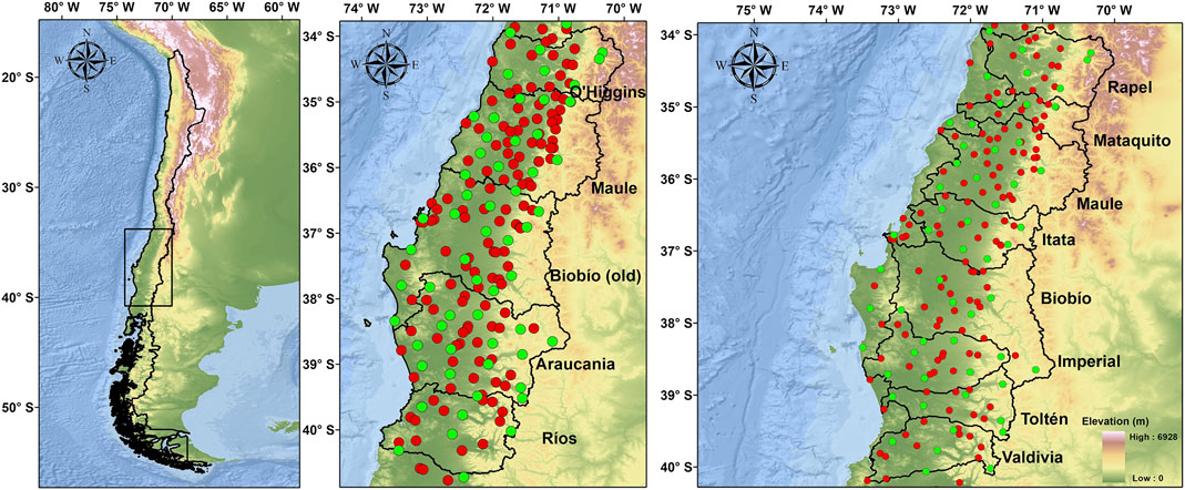
FIGURE 1. (A) Study area in central-southern Chile (O’Higgins–Los Ríos). (B) River basins used for spatial yield analysis of the weather research and forecasting model, the gridded precipitation sets (Table 2), and the topo-climatic model. The red dots indicate the 136 stations used as input for the topo-climatic model and the 60 green dots indicate the stations used for performance analysis.

2. Study Area

Variability of the South Pacific subtropical anticyclone and high-latitude pressure centers dominates Chile’s synoptic climate (Fuenzalida, 1982; Rojas, 2016). The narrow width (180 km on average) between the Pacific coast and the Andes (https://www.gob.cl/nuestro-pais/), along with a north–south extension of 4,000 km, contributes to a variety of climates (Valdés et al., 2016a). Chile holds a distinct climatic characteristic from low to high moisture from north to south. Because of the orographic effect, the main precipitation pattern shows an annual accumulation moving to the south and the Andes (Pizarro et al., 2012; Quintana and Aceituno, 2012; Valdés-Pineda et al., 2014; Valdés et al., 2016a), with annual precipitations in the north 30°S of about 100 mm increasing up to 3,000 mm in the south 40°S (Pizarro et al., 2012; Barrett and Hameed, 2017). Since elevation increases from the sea level in the west to some thousand meters in a few hundred kilometers to the east, Andean precipitation can double coastal rainfall (Viale and Garreaud, 2015; Barrett and Hameed, 2017).

Within Chile, our study area corresponds to the center-south zone of the country between latitudes $\left({34}^{\circ }\text{S–}{41}^{\circ }\text{S}\right)$, from O’Higgins to Los Ríos regions (Figure 1). This region presents a well-defined annual cycle characterized by a peak of precipitation in austral winter and lower values in austral summer (Valdés et al., 2016a; Valdés et al., 2016b). Besides, this is one area with the highest humidity in the southern hemisphere (Miller, 1976) and one of the extra-tropical areas most affected by El Niño and La Niña events (Grimm et al., 2000; Waylen and Poveda, 2002). Due to its transitional location between subtropical and high-latitude temperatures, climate is characterized by a significant interannual rainfall variability (Aceituno et al., 1993; Quintana, 2004; Le Quesne et al., 2009). The El Niño Southern Oscillation, mostly in the northern section, and the Pacific Decadal Oscillation to the south affect hydrological regimes (Arumí-Ribera and Oyarzún-Lucero, 2006; Araya-Ojeda and Isla, 2016). The south-central zone presents yearly accumulated precipitation between 100 and 3000 mm from the north to south (Quintana and Aceituno, 2012; Valdés et al., 2016a). This is a zone of active recharge for surface and groundwaters as a result of infiltration and transport processes in valleys, channels, and fractured systems in the high zones and the pre-mountain ranges (Arumí et al., 2012; Carling et al., 2012). Along the Andes, particularly toward the south, where the role of oceanic fronts is prominent, the orographic effect increases rainfall.

3. Methodology

The choice and organization of observed precipitation data are presented in Section 3.1. Section 3.2 shows the development and execution of the atmospheric model, and then the adjustment and selection (which considers the database presented in Section 3.1 of the modeled precipitation fields). The collection of global gridded precipitation sets and their later data choice are discussed in Section 3.3. Section 3.4 presents the structure and procedure in the construction of the topo-climatic dynamic model. The statistical analysis strategy required for the process of calibration and validation of the atmospheric model, choice of global gridded data and topo-climatic dynamic model, and final construction of the high-resolution gridded product is addressed in Section 3.5.

3.1. Instrumental Database

The Dirección General de Aguas and the Dirección Meteorológica de Chile (DMC) support Chile’s meteorological station network. Although these data are reliable and cover several decades, many stations are conventional (report only daily accumulation) and at low elevations (Garreaud et al., 2016). Also, in most records (Figure 2), data gaps are common (Zambrano M. et al., 2017b). Within the study zone, we initially considered 301 stations reporting daily observations (Figure 1). We eliminated stations with more than $30\text{\%}$ monthly data gaps between 2000 and 2011 (105 stations). From the remaining stations (196), 136 correspond to input for model calibration and 60 for validation.

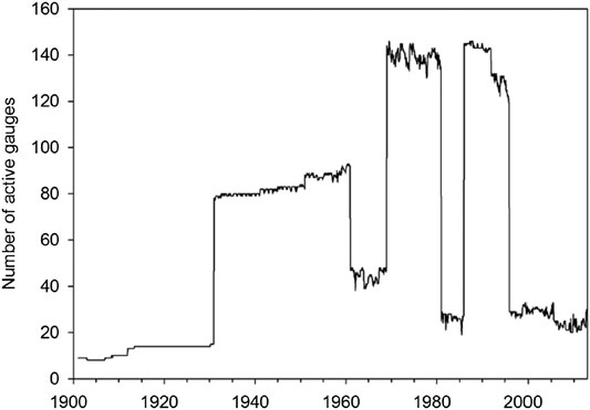
FIGURE 2. Number of precipitation stations in Chile used by Global Precipitation Climatology Centre dataset (Schamm et al., 2015). Source: Zambrano M. et al. (2017).

3.2. Atmospheric Modeling

An atmospheric numerical simulation was developed using the Weather Research and Forecasting model (WRF), version 3.6 (Skamarock et al., 2008) for the period $2000\text{–}2011$ to obtain a high-resolution robust precipitation dataset. The simulation was initialized in October 1999 and run through December 2014, with the first 3 months discarded as model spin-up. As recommended by the DMC (DMC, 2015), this model must consider a domain covering some parts of the Pacific Ocean to capture the phenomena approaching the continent (Yáñez-Morroni et al., 2018). We used three nested domains for downscaling (Figure 3). The largest domain, $D_1$, at 36 km resolution, contained two nested domains, $D_2$ and $D_3$, each with a ratio of 1/3 relative to its respective parent (Table 1). Initial and boundary conditions for the $D_1$ domain correspond to the ERA-Interim global reanalysis, at a spatial grid resolution of ${0.75}^{\circ }\times {0.75}^{\circ }$ latitude–longitude and 60 vertical hybrid levels (Dee et al., 2011). Ingestion of ERA-Interim’s atmospheric fields was every 6 hours. The twelve-year simulation took about 22 real computational months in the Troquil cluster at the Center of Excellence of Scientific Modeling and Computing at Universidad de La Frontera. In atmospheric numerical simulations, parameterizations strongly influence the patterns of simulated precipitation (Wang and Seaman, 1997; Gallus and William, 1999; Jankov et al., 2005) and also affect model response to changes in grid spacing (Gallus and William, 1999) or soil moisture (Gallus and William, 1999; Gallus et al., 2000). A summary of the settings used is shown in Table 1, selected following recommendations of the DMC (DMC, 2015).

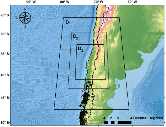
FIGURE 3. Display of the domains used in weather research and forecasting model. D₁: parent domain with 36-km resolution. D₂: first nesting with 12-km resolution (1/3 parent domain size). D₃: second nesting, with 4-km resolution (1/9 parent domain size).

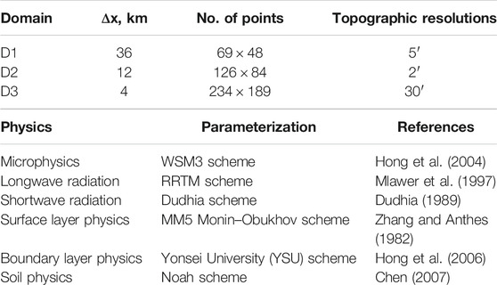
TABLE 1. Domain configuration and parameterization schemes selected for the weather research and forecasting model.

We implemented a method for systematic error correction (bias) applied to every WRF’s generated precipitation field within each regional domain (Figure 1A). We calculated the relationship between the average monthly precipitation of a station and its nearest grid point of the WRF model (a virtual station). For each regional domain, Eq. 1 determined selection of WRF’s virtual stations. Next, we obtained and applied a fit factor $\mu \left(P_o^s\right)/\mu \left(P_{wrf}^s\right)$ to each grid point in the region (Eq. 1). Finally, each adjusted grid point was reevaluated and discarded as input to the dynamic topo-climatic model if it did not meet the requirement of Eq. 1.

where $P_{min}^o$ and $P_{max}^o$ are the minimum and maximum observed rainfall, respectively; $\mu \left(P_o^s\right)$ is the monthly observed average of stations; $\mu \left(P_{wrf}^s\right)$ is the monthly average of the nearest virtual stations delivered by the WRF model; $P_{wrf}$ is the computed gridbox; and $P_{wrf}^{cs}$ is the bias-corrected precipitation.

3.3. Global Gridded Datasets

Our compilation includes eight precipitation products from diverse sources (observation, reanalysis, satellite, or mix) and present different spatial and temporal resolutions, and coverage (semiglobal or global, Table 2). We did not bias-correct these precipitation products as this was performed by the teams that built them. Therefore, each product’s dynamics depends entirely on its source. Three precipitation sets were based on satellite data ($\text{TRMM}$, $\text{CMOPRH}$, and $\text{SM}2\text{RAIN}$), one set was based exclusively on observed data ($\text{CRUv}4.01$), and four sets were built with satellite data, reanalysis, and observations ($\text{PGFv}3$, $\text{CHIRPSv}2.0$, $\text{PERSIANN}-\text{CDR}$, and $\text{MSWEPv}1.2$).

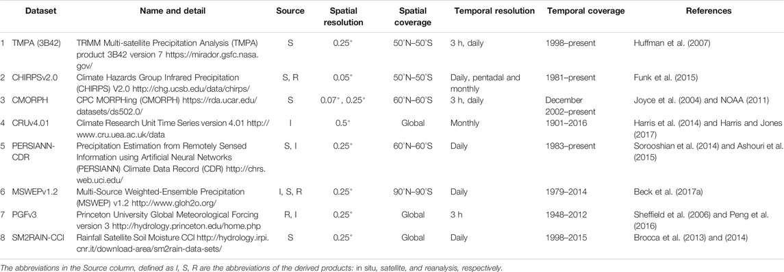
TABLE 2. Description of the 8 (quasi) global (sub-)precipitation grids used in this study.

In order to minimize the difference in bias from these precipitation products (Zhang et al., 2019; Yeh et al., 2020), each gridded precipitation product used in this study was evaluated according to Eq. 2, where every point was discarded when it was either under or over $5\text{\%}$ of the respective minimum and maximum precipitation observed within the respective regional domain (Figure 1A). This procedure tries to cover areas where atmospheric modeling precipitation grids are discarded (see Section 3.2). Thus, once the best set for each regional domain was obtained, no overlap of data with the WRF model was sought. Otherwise, that is, if overlap happens, the one with the smallest difference in minimum and maximum precipitation bias is selected according to Eq. 2. Note that if neither atmospheric nor the gridded data met the admissibility conditions, that place is not used.

where $P_g$ is the precipitation gridbox of each set in Table 2, $P_g^s$ is the selected gridbox of the grid set, and $P_{min}^o$ and $P_{max}^o$ are the minimum and maximum precipitation of each subregion, respectively. Otherwise, we delete this gridbox.

3.4. Dynamic Topo-Climatic Model

Our model is a multiple linear regression between precipitation as the dependent variable (Swain et al., 2017; Navid and Niloy, 2018; Devi et al., 2020) and the following independent variables: elevation, slope, exposure, continentality, latitude, and longitude (Zambrano, 2011; Camera et al., 2014; Cifuentes, 2017). The model fits the observed values by a least square procedure between the observed and predicted values (Delbari et al., 2019). The linear dependence function is given by

where α is the intercept, and the values ${\beta }_i,i=1,\mathrm{.},p$ are called regression coefficients associated with the variables elevation $\left(\text{elev}\right)$, exposure $\left(\text{exp}\right)$, slope $\left(\text{slp}\right)$, continentality $\left(\text{cont}\right)$, latitude $\left(\text{lat}\right)$, and longitude $\left(\text{lon}\right)$.

To get the dataset gridded at 800 m, we used the Shuttle Radar Topography Mission digital elevation model (Farr et al., 2007) at 90-m spatial resolution. This digital elevation model is aggregated to an 800-m resolution (Figure 4). Note that the model domain covers five administrative regions: O’Higgins, El Maule, Biobío (now Biobío and Ñuble), La Araucanía, and Los Ríos (Figure 1A). However, the domains correspond to regional boundaries (Figure 1A), along with a $25\text{\%}$ increase in the contribution from the neighboring regions. With this, we ensured that basins shared between different regions are covered. Also, mutual covering between domains ensures greater consistency and homogeneity to the global solution. Each month, data used for the construction of the field change with input data (Sections 3.2 and 3.3).

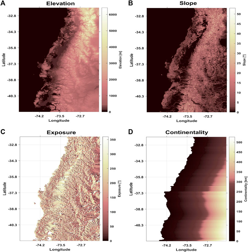
FIGURE 4. Digital terrain model with independent variables: (A) elevation, (B) slope, (C) exposure, and (D) continentality.

For each regional domain, we solve the topo-climatic model monthly, trying different configurations of the independent variables described in Eq. 3. We carry out tests in which either a single topographic variable or a set of them is eliminated. Thus, each month, six $\left(6!\right)$, different tests can be performed. The structure is tested monthly, and at the end of the 12-year period (144 months), the most effective model is used as the basis for the calculation of the monthly topo-climatic model coefficient. Because it plays a significant role in a topo-climatic model, elevation is the only variable used in all calculations. Similarly, the different tests indicated that the elevation and exposure variables are necessary for all regional domains. In the following, only the most representative models are shown.

Each model developed is labeled according to the variables in Eq. 3: $\left(all\right)$, all the variables; $\left(wexp\right)$, without exposure; $\left(wslp\right)$, without slope; $\left(wlat\right)$, without latitude; $\left(wlon\right)$, without longitude; and $\left(wcon\right)$, without continentality variable. Subsequently, each model was evaluated through an analysis of variance (ANOVA) test and a residual analysis. We use different statistics to determine the most appropriate structure for each regional domain, namely, the standardized standard deviation (${\sigma }_e$, Eq. 6), standardized mean square error ($nmrse$, Eq. 7), percentage of the standardized systematic error ($pbias$, Eq. 9), correlation coefficient (${\rho }_{xy}$, Eq. 8), Nash–Sutcliffe coefficient ($nse$, Eq. 10), and the modified Willmott coefficient (d, Eq. 11).

Figure 5 depicts the three phases carried out for the construction of the dynamic topo-climatic model. The first phase $\left(F1\right)$ determines the number of local precipitation stations and their subsequent selection (Section 3.1). The second phase $\left(F2\right)$ corresponds to climatic modeling that produces precipitation fields, which are then bias-corrected (Section 3.2) using the local data (Section 3.1). The third phase $\left(F3\right)$ (Section 3.3) selects the global precipitation gridded sets which are used alternatively for the locally adjusted precipitation modeled fields. Finally, within the fourth phase $\left(F4\right)$ (Section 3.4), on each geographical domain, the tests allow the choice of the coefficients of variables (elevation, slope, exposure, continentality, latitude, and longitude) to develop the high-resolution fields.

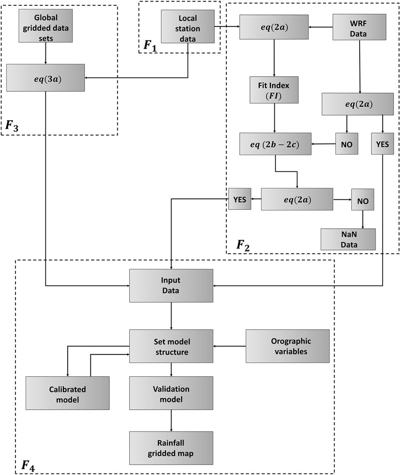
FIGURE 5. Schematic overview of the dynamic topo-climatic model development.

3.5. Statistical Analysis

This section presents the statistical analysis strategy required for the atmospheric model correction and adjusting process, global gridded dataset selection, the topo-dynamic model calibration and validation, and the final high-resolution gridded product construction.

Spatial fitting, selection of monthly fields from the WRF model, and spatial selection of the best monthly products of global grid precipitation are analyzed for each regional domain (Figure 1A): The results of these processes are displayed for eight hydrological basins (Figure 1B). Our strategy uses a range of statistics following Cardoso et al. (2013), Ji et al. (2015), and Akhter et al. (2019): standardized standard deviation (${\sigma }_e$, Eq. 6), standardized mean square error ($nrmse$, Eq. 7), correlation coefficient (${\rho }_{xy}$, Eq. 8), percentage of the standardized systematic error ($pbias$, Eq. 9), Nash–Sutcliffe coefficient ($nse$, Eq. 10), and modified Willmott coefficient (d, Eq. 11). We used six indices in the data comparison because each of them quantifies only one aspect of data agreement or disagreement.

Once the selection of the best grid points is completed, a different monthly topo-climatic model is constructed over each regional domain. For this process, a calibration phase is followed by a validation phase. As previously indicated, we used $70\text{\%}$ of the local rainfall data $\left(136\text{\hspace{0.17em}stations}\right)$ for calibration and $30\text{\%}$$\left(60\text{\hspace{0.17em}stations}\right)$ for validation. In both processes, due to the stations’ inhomogeneous distribution and notorious inadequate coverage in mountainous areas, the spatial distribution of the local stations chosen tried to maximize homogeneous coverage of each regional domain.

Calibration of the dynamic topo-climatic model includes application of an ANOVA test, and the goodness-of-fit parameters $R^2$ (Eq. 4) and $R_j^2$ (Eq. 5) with the respective residual analysis. For the validation stage, the following statistics are used: standardized standard deviation (${\sigma }_e$, Eq. 6), standardized mean square error ($nrmse$, Eq. 7), correlation coefficient (${\rho }_{xy}$, Eq. 8), percentage of the standardized systematic error ($pbias$, Eq. 9), Nash–Sutcliffe coefficient ($nse$, Eq. 10), and the modified Willmott coefficient (d, Eq. 11). We also analyze results using Taylor’s diagrams (Taylor, 2001), to visualize results model behavior relative to observations in terms of the spatial structure generated by the Pearson correlation coefficient $\left({\rho }_{xy}\right)$, standardized mean square error ($nrmse$), and absolute standardized standard deviation $\left(\left|{\sigma }_e\right|\right)$. Also, we used boxplot diagrams to visualize standard deviation scores $\left({\sigma }_e\right)$, the mean systematic error percentage $\left(pbias\right)$, coefficient of Nash–Sutcliffe ($nse$), and modified Willmott coefficient (d). This calibration and validation processes are performed monthly, thus generating every month a different topo-climate model. Calibration and validation results presented here correspond to the average of all these months. Also, given that the whole domain includes a climatic transition zone, the results of the eight basins are summarized in three subdivisions: northern, central, and southern areas (Figure 1B).

The statistics used are defined in the following equations:

where X and Y are observed and simulated precipitation, respectively.

4. Results

In Sections 4.1 and 4.2, the average precipitation behavior of the adjusted atmospheric model (see Section 3.2) and the selected global gridded products (see Section 3.3) is presented over three zones (north, center, and south), covering eight basins (Figure 1B). All local stations (196) are used, and these are presented using Taylor and boxplot diagrams (see Section 3.5). Section 4.3 presents the best results associated with the calibration process of the dynamic topographic-climatic model within each regional domain (Section 4.3.1) using 132 precipitation stations (Section 3.1). The model validation stage of the chosen model using 60 stations in Section 4.3.2 is presented for the eight basins (Figure 1B). This part of the article ends by showing the annual accumulation of the constructed monthly climatology.

4.1. Atmospheric Model

In the northern zone (Figures 6A-C), ${\rho }_{xy}$ shows an average of 0.85, but we can appreciate atypical cases with values below 0.65. Meanwhile, $nmrse$ shows agreements close to 0.65, although all basins present cases above 0.5. For ${\sigma }_e$ (Figure 7A), the average agreement is close to 0.1, with Rapel showing some cases above 0.3. Finally, $pbias$ (Figure 7B) gives an average agreement of $14\text{\%}$, with Mataquito presenting the lowest values since $75\text{\%}$ of the analyzed stations there are close to $10\text{\%}$.

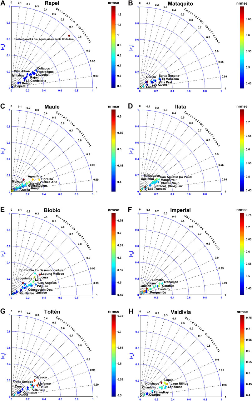
FIGURE 6. Taylor’s diagrams corresponding to weather research and forecasting model performance (Table 1) once fitted (Eq. 1) in basins: (A) Rapel, (B) Mataquito, (C) Maule, (D) Itata, (E) Biobío, (F) Imperial, (G) Toltén, and (H) Valdivia.

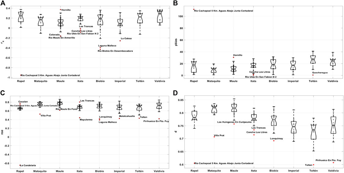
FIGURE 7. Box diagrams corresponding to the fit of the weather research and forecasting model, once adjusted (Eq. 1) on the river basins of the area under study (Figure 1B). (A) Standardized standard deviation $\left({\sigma }_e\right)$, (B) percentage of the systematic error $\left(pbias\right)$, (C) Nash–Sutcliffe coefficient $\left(nse\right)$, and (D) Willmott coefficient $\left(d\right)$.

Results for the central zone (6D,E) indicate an average for ${\rho }_{xy}$ of 0.83 and 0.55 for $nrmse$, although with several cases well above 0.65. For ${\sigma }_e$ (Figure 7A), average is 0.14, with the Biobío basin showing values above 0.25. For $pbias$ (Figure 7B), the $17\text{\%}$ average is punctuated by certain basins exceeding $25\text{\%}$.

Good estimation for ${\rho }_{xy}$ characterizes the southern region (Figures 6F-G), averaging a value of 0.87. Within this region, Valdivia shows cases close to 0.6. $nrsme$ exhibits an average of 0.56, although all basins have cases above 0.7. In turn, ${\sigma }_e$ (Figure 7A) shows an average of 0.15, with Imperial and Toltén above 0.3. Finally, $pbias$ (Figure 7B) shows an average of $9\text{\%}$. Toltén gives the lowest average estimate with $7\text{\%}$.

We show the $nse$ and Willmott coefficient $\left(d\right)$ results in all regions (and basins) in Figure 7D. In all basins, the average value for $nse$ is greater than 0.7; only Rapel and Maule show values smaller than 0.6. The Willmott coefficient (d) shows values close to 0.8 in the north zone (Rapel, Mataquito, and Maule) and a value of 0.75 for the central zone (Itata and Biobío), whereas for the southern zone (Imperial, Toltén, and Valdivia) $25\text{\%}$ of stations show values below 0.75 with a large spread.

4.2. Global Precipitation Datasets

In the northern zone (Figures 8A-C), ${\rho }_{xy}$ presents an average value of 0.74. However, $\text{CMORPH}$ and $\text{SM}2\text{RAIN}$ show ${\rho }_{xy}$ values under 0.6 in all zones. Variations in $nrmse$ show an average of 0.4, with Mataquito and Maule displaying 0.5 for the $\text{PERSIAN}$ dataset. For ${\sigma }_e$, the average is 0.27, while for $\text{CMORPH}$ and $\text{SM}2\text{RAIN}$ the values are higher than 0.6 for the whole zone (Figure 9A). $pbias$ (Figure 9B) shows an average of $20\text{\%}$, with anomalous estimates (over $30\text{\%}$) in Mataquito and Maule.

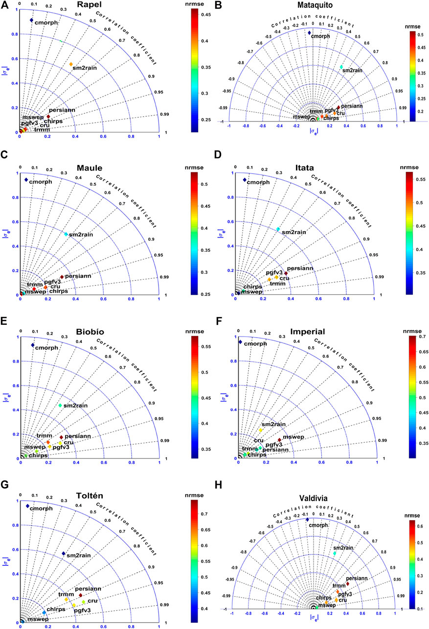
FIGURE 8. Taylor’s diagrams corresponding to the gridded set performance (Table 2), once fitted (Eq. 2) on the river basins of (A) Rapel, (B) Maule, (C) Itata, (D) Biobío, (E) Imperial, (F) Toltén, (G) Mataquito, and (H) Valdivia.

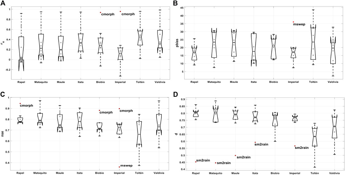
FIGURE 9. Box diagrams corresponding to the gridded set performance (Table 2), once adjusted (Eq. 2) on the river basins of the area under study (Figure 1B). (A) Standardized standard deviation $\left({\sigma }_e\right)$, (B) percentage of the systematic error $\left(pbias\right)$, (C) Nash–Sutcliffe coefficient $\left(nse\right)$, and (D) Willmott coefficient $\left(d\right)$.

Over the central zone (Figures 8D,E), ${\rho }_{xy}$ presents an average of 0.74. Again, $\text{CMORPH}$ and $\text{SM}2\text{RAIN}$ show the worst results for ${\rho }_{xy}$, with scores under 0.6. Meanwhile, $nrsme$ gives an average of 0.44, although the entire area shows values above 0.3. Continuing with ${\sigma }_e$ (Figure 9A), the average is 0.34. As above, $\text{CMORPH}$ and $\text{SM}2\text{RAIN}$ give estimates fairly different relative to the average, higher than 0.5. Here, $pbias$ (Figure 9B) shows an average error of $20\text{\%}$, while the highest estimates are below $30\text{\%}$ in the Itata and Biobío basins.

For the southern zone (Figures 8F-H), ${\rho }_{xy}$ shows an average of 0.73. Similar to that described in the previous paragraph, $\text{CMORPH}$ and $\text{SM}2\text{RAIN}$ show the worst results with estimates for ${\rho }_{xy}$ under 0.6. A high $nrmse$ in all basins delivers an average of 0.48. $\text{MSWEP}$ and $\text{PERSIAN}$ show the highest $nrmse$ with values above 0.6. The average ${\sigma }_e$ is 0.34, with $\text{CMORPH}$ and $\text{SM}2\text{RAIN}$ above 0.6 (Figure 9A). Meanwhile, $pbias$ (Figure 9B), exhibits an average of $20\text{\%}$. In this case, it is important to highlight that in all basins, the different datasets present errors more significant than $30\text{\%}$.

The Nash–Sutcliffe ($nse$) and Willmott (d) coefficients are displayed for all basins (Figures 9C,D). Here, $nse$ shows a mean adjustment of about 0.6 from the Rapel to the Imperial basin. There is a larger spread for Toltén and Valdivia, with the minima below 0.55. The Willmott coefficient (d) exhibits a similar distribution from Rapel to Imperial, with almost $90\text{\%}$ of the datasets above 0.7. We again see more heterogeneity in the Toltén and Valdivia basins with values below 0.5. $\text{SM}2\text{RAIN}$ shows the weakest performance for all basins.

4.3. Dynamic Topo-Climatic Precipitation

4.3.1. Regional Domain Analysis

The average fit of the dynamic topo-climatic model for each regional domain is shown in Figure 10. The coefficient of determination $\left(R^2\right)$ (Figure 10A) shows an excellent model performance in O’Higgins and Biobío regions with values above 0.8 and in Araucanía and Los Ríos regions with values below 0.77. The adjusted coefficient of determination $\left(R_j^2\right)$ (Figure 10B) also shows skilled fitting (over 0.8) from O’Higgins to Biobío regions, although the Maule basin shows the lowest estimate for $R_j^2$. The same occurs in Araucanía and Los Ríos regions. The $F_{\text{value}}$ from the ANOVA shows an excellent fit of the model with a $P_{\text{value}}$ less than 0.05 (Figure 10C). In turn, the average model performance for ${\rho }_{xy}$ is higher than 0.9 in all domains (Figure 10H). We also find an average $pbias$ below $22\text{\%}$, with O’Higgins and Biobío below $15\text{\%}$ (Figure 10F). The outliers identified for ${\sigma }_e$ (Figure 10G) exhibit an error below 0.22, supporting that the model is skilled. $nrmse$ (Figure 10E) shows average model values below 0.4, while values above 0.48 are shown in Araucanía and Los Ríos. In these regions, a high error confirms the model is more uncertain in estimating extreme precipitation events. Table 3 shows the results for the calibrated model configuration ($R^2$, $R_j^2$, $F_{\text{value}}$, and $P_{\text{value}}$) and error estimate (${\sigma }_e$, $nrmse$, $pbias$, and ${\rho }_{xy}$) for each regional domain.

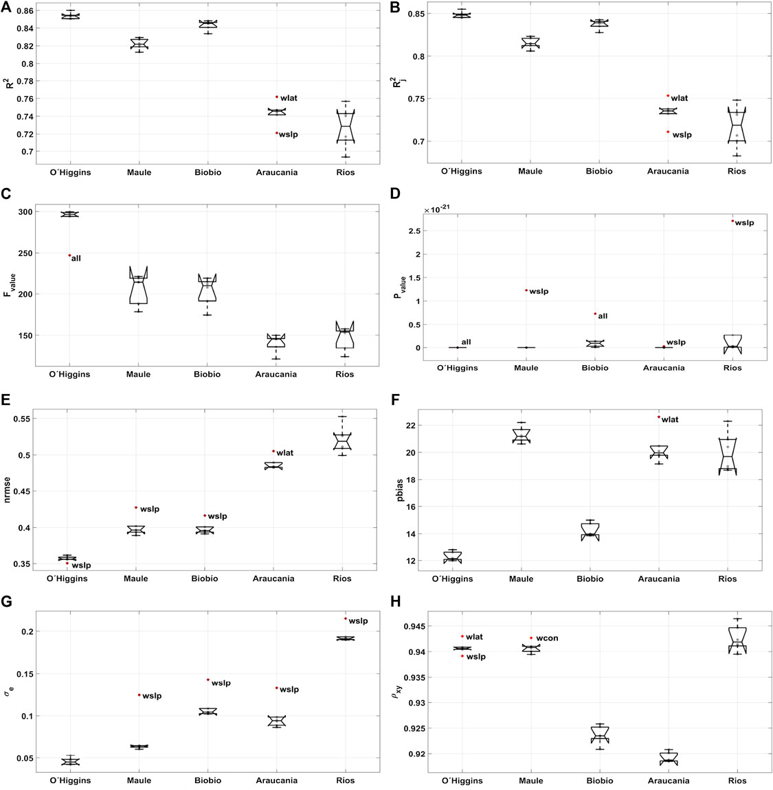
FIGURE 10. Box diagrams corresponding to the adjustment of the topo-climatic model on the domains in execution. (A) Multiple determination coefficient $\left(R^2\right)$, (B) adjusted multiple determination coefficient $R_j^2$, (C) value F, (D) value P, (E) standardized mean square error $\left(nrmse\right)$, (F) percentage of systematic error $\left(pbias\right)$, (G) standardized standard deviation $\left({\sigma }_e\right)$, (H) Pearson correlation coefficient $\left({\rho }_{xy}\right)$.

4.3.2. Zonal and Basin Analysis

The northern zone (Figures 11A-C) shows an average ${\rho }_{xy}$ of 0.88, although some stations in Rapel get values close to 0.6. Meanwhile, the $nrmse$ exhibits an average of 0.46, although in Rapel and Maule some cases are above 0.55. Interestingly, ${\sigma }_e$ (Figure 12A) shows an average fit of 0.07, with that in Maule below $-0.4$. $pbias$ (Figure 12B) shows an average adjustment of $18\text{\%}$, but Rapel and Maule show the most considerable difference with an estimate over $50\text{\%}$.

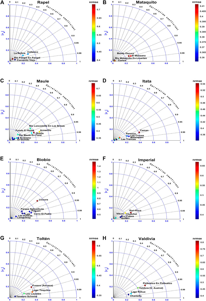
FIGURE 11. Taylor diagrams corresponding to the performance of the topo-climatic model on the river basins (Figure 1B): (A) Rapel, (B) Mataquito, (C) Maule, (D) Itata, (E) Biobío, (F) Imperial, (G) Toltén, and (H) Valdivia.

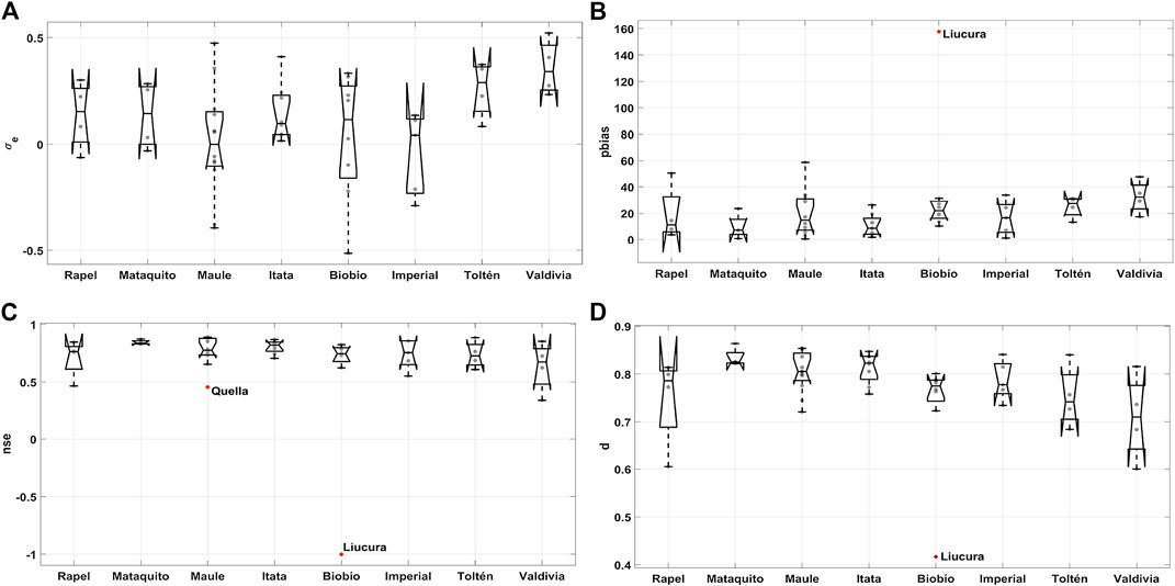
FIGURE 12. Box diagrams corresponding to the adjustment of the topo-climatic model on the domains in execution. (A) Standardized standard deviation $\left({\sigma }_e\right)$, (B) percentage of the systematic error $\left(pbias\right)$, (C) Nash–Sutcliffe coefficient $\left(nse\right)$, and (D) Willmott coefficient $\left(d\right)$.

The central zone (Figures 11D,E), ${\rho }_{xy}$ shows an average of 0.89 and Biobío exhibits values below 0.8. The $nrmse$ displays an average of 0.52, while Biobío shows an irregular value greater than 1. The average for ${\sigma }_e$ is 0.1 (Figure 12A) with only Biobío being below $-0.5$. For $pbias$ (Figure 12B) there is a $24\text{\%}$ average error with Biobío showing an estimate below $100\text{\%}$.

The southern zone (Figures 11F-H) exhibits an average ${\rho }_{xy}$ over 0.9, while the lowest estimates are above 0.85. $nrsme$ shows an average of 0.52, with all basins having some values above 0.66. On the other hand, while ${\sigma }_e$ (Figure 12A) shows an average of 0.1, only the Imperial basin exhibits a low estimate of $-0.2$. $pbias$ (Figure 12B) shows an average of $24\text{\%}$. $nse$ shows an average above 0.7 in all basins (Figure 12C); only two atypical cases are detected in Maule and Biobío with values of 0.5 and $-1$, respectively. On the other hand, d (Figure 12D) shows an average fitting of 0.75. Only Biobío exhibits an outlier in the Liucura station with a value below 0.5.

On each regional domain, a different monthly model is adjusted to the calibration data and checked using validation points. This allows us to construct a monthly solution for each regional domain, delivering a dataset of monthly fields covering the period $2000\text{–}2011$ that subsequently are used to produce monthly climatologies from January to December. Figure 13 shows the observed accumulated annual rainfall and the one obtained by the topo-climatic dynamic model over the study area $\left({34}^{\circ }\text{S}–{41}^{\circ }\text{S}\right)$. Figure 13B indicates an adequate distribution of precipitation from north to south and from the ocean to the Andes. There is a progressive increase from north to south and drastic increases in mountain areas, particularly along the Andes and the coastal cordillera. Thus, in sectors close to the coast (from ${38}^{\circ }\text{S}$), an abundant annual precipitation is identified, sometimes reaching over 2,000 mm. Throughout the Andean areas, the accumulated annual rainfall can reach and exceed 3,000 mm per year. Finally, between the coast and the Andes below ${36}^{\circ }\text{S}$, it is possible to identify a decrease in annual precipitation.

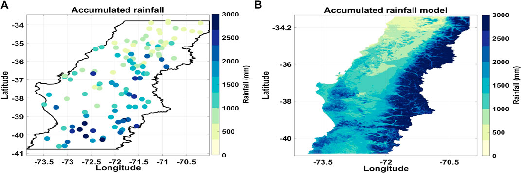
FIGURE 13. Annual cumulative rainfall. (A) Rainfall observed and (B) dynamic topo-climatic model.

5. Discussion and Conclusion

High-resolution precipitation spatial variability is significant in different fields such as hydrology, environment, forestry, and agriculture. In Chile, several authors worked on gridded precipitation datasets built only with the information available from local stations in some areas of the country (Román and Andrés, 2010; Jacquin and Soto-Sandoval, 2013; Reyes, 2013; Castro et al., 2014; Sijinaldo, 2015). Also, in some cases, datasets were generated from observed data and low-resolution gridded data higher than ${0.25}^{\circ }$ (Morales-Salinas et al., 2012) or even poorer quality datasets. Thus, these high-resolution datasets are inadequate to study large areas and/or the whole country. Moreover, the insufficient spatial distribution of the pluviometric network (Muñoz et al., 2018) precludes real hydro-climatic impact under current environmental conditions.

Therefore, we assert that the dataset will be useful for different communities in Chile. It will be useful for agricultural, forestry, and livestock planning, for example, and for national institutions such as the Dirección General de Aguas (DGA), the Instituto de Investigaciones Agropecuarias (INIA), and the Instituto Forestal de Chile (INFOR), among others. This product can serve as a basis of comparison for studies aimed at investigating future climate or agricultural changes (Orrego et al., 2016), allowing investigation of the role of and Antartic Oscillation and many climatic phenomena on some local precipitation-related aspects (Fustos et al., 2020b), which is beyond the scope of this study.

To get an improved dataset and to quantify precipitation, we built a high-resolution dynamic statistical gridded precipitation product at $\sim 800\text{\hspace{0.17em}m}$. Its development involved time series of local precipitation and different global precipitation grid sets (as shown in Table 2). To detect spatial-temporal variability of precipitation, we performed numerical modeling of the atmosphere over the study area at 4 km spatial resolution for the period $2000\text{–}2011$. These outputs are a powerful tool for statistical scale reduction (Widmann et al., 2003; Schmidli et al., 2006; González-Rojí et al., 2019). Also, within each region, according to Eqs. 1and2 requirements, we performed a month-by-month data selection. We also evaluated precipitation time series belonging to eight basins to estimate the responses of the best products that entered our dynamic topo-climatic model (Figure 11).

We evaluated some precipitation grids and the results are presented in Table 2. To classify the optimal precipitation estimates and reduce uncertainty, we used a selection criterion (Eq. 2). As shown by Zambrano F. et al. (2017) and Zambrano M. et al. (2017), the performance of many is unsatisfactory. The products $\text{CHIRPS}$, $\text{MSWEP}$, and $\text{PGFv}3$ show the most accurate estimations $\left({\rho }_{xy}>0.8\right)$. Meanwhile, $\text{CMORPH}$ and $\text{SM}2\text{RAIN}$ provide the worst performance over the whole study area $\left(<0.6\right)$, and the average of ${\sigma }_e$ displays a similar distribution in all basins. However, the $\text{CMORPH}$ set exhibits the highest mismatches, with estimates close to 1 in Biobío and Imperial. $pbias$ shows a similar distribution along all basins between $10$ and $30\text{\%}$. The Nash–Sutcliffe coefficient ($nse$) shows a decreasing yield from Rapel to Itata $\left(>0.7\right)$ along with an increasing dispersion. For example, at Biobío and Imperial, the adjustment is centered on 0.7 with low dispersion. Also, Toltén and Valdivia have an average of 0.7, but with high dispersion. On the other hand, Willmott (d) does not show an improvement in the performance of the datasets, although it shows a similar pattern as $nse$$\left(>0.7\right)$. For all basins, we notice that $\text{SM}2\text{RAIN}$ shows low values. However, model fitting results for some datasets should be seen with caution, since we eliminated any value above or below $5\text{\%}$ of the respective maximal or minimal observed precipitation. Therefore, cleaned data improve the estimates of these sets.

Atmospheric dynamic models, like WRF, simulate precipitation based on convective and large-scale processes (such as precipitation from cumulonimbus fronts or clouds), generating an improved distribution of precipitation as well as other fields such as temperature (Pope and Stratton, 2002; Jung et al., 2006; Gent et al., 2010). However, there are still errors attributed to feedback processes, which are not necessarily reduced by increasing the model spatial resolution. As these errors are pronounced on rough terrain, and even more so in mountainous areas, to take that possibility into account, it was necessary to add a $5\text{\%}$ correction. Despite this, the limited density of observation along the Andes incorporates a high degree of uncertainty, preventing homogeneous fit, thus making the construction of a correct model at high altitude difficult. Taylor and boxplot diagrams show that the model presents a remarkable performance in the northern zone (Figures 6, 7). As far as the central zone is concerned, adequate fitting is again obtained for ${\rho }_{xy}$, $nse$, and d.

To construct our dynamic geostatistical model, we used global precipitation grids and a local atmospheric model (Table 2) in addition to regional domains (Figure 1B). This is a nontrivial process, particularly in regions with a great variety of space–time patterns (Zhang et al., 2016). During the precipitation reconstruction phase, we verified the elevation coefficients relative to each regional domain with available local information. For the mountains, the little local information available prevents adequate correction and adjustment of the WRF model or the gridded data. Consequently, in the heights, the precipitations should generally be overestimated. Each month, the adjustment provides different elevation coefficients for each regional domain. However, for the entire domain, the solution that imposed a single elevation coefficient, considering all the information from north to south, turned out to be the best.

The results of the model chosen for each region (Table 3) show reasonable skill in the assessed basins (Figures 11, 12). However, the model is unable to satisfactorily represent extreme precipitation events, which gradually increase from north to south. It is essential to note that the choice of the regression model is conditioned by the input data selection and the domain used. Only numerical modeling and satellite information are the ones that provide adequate spatial coverage and persistence. In turn, statistical downscaling can improve the accuracy of discrete meteorological measurements (Diez et al., 2005; Fernández-Ferrero et al., 2009; Le Roux et al., 2018; González-Rojí et al., 2019). To our knowledge, this kind of study is scarce in Chile, not only in the construction of grilled climatic data but also in the analysis and comparison of different methodologies for an optimal statistical scale reduction model or the domain type needed to carry this out.

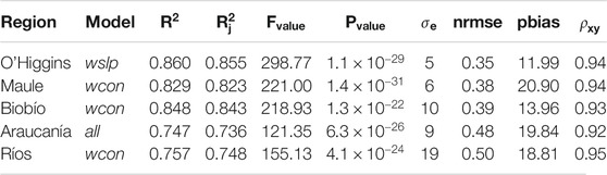
TABLE 3. Statistical summary of the type of topo-climatic model chosen by the political domain of each region. (wslp), (wcost), (all), (wcon).

The database presented in this study results from atmospheric modeling, corrected, adjusted, and ported to higher resolution by a dynamic topo-climatic method using data from local meteorological stations and satellite fields. Note that to improve the accuracy of database selection by different statistical methodologies, we visually inspected each dataset in detail and month by month. However, we still depend on the quality of the atmospheric modeling, which is not reality, and that of the satellite fields and local data. Therefore, we would like to point out that although we are confident that the method used and the resolution will allow a better understanding of local hydrological variability, this database does not replace reality. That is why, contrary to several global gridded databases, which do not stipulate it, we recommend within each basin to check against local data and correct any existing bias.

Of course, there are still many improvements to be made. Note that we will always be dependent on the distribution of the local weather network, which is the only one that allows the calibration and validation process. It is fundamental to improve the quality in many places, notably in the slopes of the Coastal and Andean mountain ranges, where weather coverage is almost nonexistent. A nonhomogeneous distribution of altitude data, used to build a solution over the mountains, may not represent the different mechanisms in both cordilleras, sometimes separated by less than 100 km. Thus, specific measurement campaigns are needed to support, for example, model calibration during brief periods and on a local scale. However, many phenomena throughout Chile develop at high frequencies, where the monthly value does not allow for a correct description (Fustos et al., 2020a). Thus, while it is necessary to expand time–space coverage, north–south and up to 2020, in addition to build other high-resolution grids of essential hydro-climatic parameters (such as temperature), it is also imperative to focus on daily grid products.

Data Availability Statement

The datasets generated for this study are available on request to the corresponding author.

Author Contributions

RA assisted the first author (FA) at different levels of research, such as conception, design, analysis, and editing of the manuscript. Although RA is responsible for the overall concept and design of the research, data collection, development of atmospheric modeling, and statistical analysis of this manuscript was performed by FA; RA and AA contributed to the technical implementation required for atmospheric modeling; and AA improved the mathematical interpretation of the results and participated in the review of the submitted manuscript.

Conflict of Interest

The authors declare that the research was conducted in the absence of any commercial or financial relationships that could be construed as a potential conflict of interest.

Acknowledgments

We appreciate and are indebted to both the reviewers’ outstanding work, whose rigor and scientific culture helped us improve both form and substance. We are very grateful and indebted to our colleague A. Fernandez, for careful proofreading of the manuscript. We are also grateful for advices by B. Mark. We are grateful for funding support received from the PhD in Physical Sciences program from the Faculty of Physical and Mathematical Sciences, the Research Directorate (DRINV), and Postgraduate Directorate of the University of Concepción. This research was partially supported by the supercomputing infrastructure of the NLHPC (ECM-02) at Centro de Modelación y Computacion Científica, Universidad de La Frontera, CMCC-UFRO.

References

Abatzoglou, J. T. (2013). Development of gridded surface meteorological data for ecological applications and modelling. Int. J. Climatol. 33, 121–131. doi:10.1002/joc.3413
Aceituno, P., Fuenzalida, H., and Rosenblüth, B. (1993). “Climate along the extratropical west coast of south America,” in Earth system responses to global change. Editors H. A.Mooney, E. R.Fuentes, and B. I.Kronberg, (San Diego, CA: Academic Press), 61–69.
Akhter, J., Das, L., Meher, J. K., and Deb, A. (2019). Evaluation of different large-scale predictor-based statistical downscaling models in simulating zone-wise monsoon precipitation over India. Int. J. Climatol. 39, 465–482. doi:10.1002/joc.5822
Araya-Ojeda, M., and Isla, F. I. (2016). Variabilidad hidrológica en la región del biobío: los eventos el niño en zonas templadas de Chile. Revista Universitaria de Geografía 25, 31–55.
Arumí-Ribera, J., and Oyarzún-Lucero, R. (2006). Las aguas subterráneas en Chile. Bol. Geol. Min. 117, 37–45
Arumí, J. L., Rivera, D., Muñoz, E., and Billib, M. (2012). Interacciones entre el agua superficial y subterránea en la región del bío bío de Chile. Obras y proyectos., 4–13. doi:10.4067/s0718-28132012000200001. “https://www.researchgate.net/publication/241157980_Las_aguas_subterraneas_en_Chile/stats” and “https://dialnet.unirioja.es/servlet/articulo?codigo=1710339”
Ashouri, H., Hsu, K.-L., Sorooshian, S., Braithwaite, D. K., Knapp, K. R., Cecil, L. D., et al. (2015). Persiann-CDR: daily precipitation climate data record from multisatellite observations for hydrological and climate studies. Bull. Am. Meteorol. Soc. 96, 69–83. doi:10.1175/bams-d-13-00068.1
Barrett, B. S., and Hameed, S. (2017). Seasonal variability in precipitation in central and southern Chile: modulation by the South Pacific High. J. Clim. 30, 55–69. doi:10.1175/JCLI-D-16-0019.1
Beck, H. E., Van Dijk, A. I., Levizzani, V., Schellekens, J., Gonzalez Miralles, D., Martens, B., et al. (2017a). Mswep: 3-hourly 0.25 global gridded precipitation (1979-2015) by merging gauge, satellite, and reanalysis data. Hydrol. Earth Syst. Sci. 21, 589–615. doi:10.5194/hess-21-589-2017
Beck, H. E., Vergopolan, N., Pan, M., Levizzani, V., Van Dijk, A. I., Weedon, G. P., et al. (2017b). Global-scale evaluation of 22 precipitation datasets using gauge observations and hydrological modeling. Hydrol. Earth Syst. Sci. 21, 6201–6217. doi:10.5194/hess-21-6201-2017
Berezowski, T., Szcześniak, M., Kardel, I., Michałowski, R., Okruszko, T., Mezghani, A., et al. (2016). CPLFD-GDPT5: high-resolution gridded daily precipitation and temperature data set for two largest polish river basins. Earth Syst. Sci. Data. 8, 127–139. doi:10.5194/essd-8-127-2016
Brinckmann, S., Krähenmann, S., and Bissolli, P. (2016). High-resolution daily gridded data sets of air temperature and wind speed for Europe. Earth Syst. Sci. Data. 8, 491–516. doi:10.5194/essd-8-491-2016
Brocca, L., Ciabatta, L., Massari, C., Moramarco, T., Hahn, S., Hasenauer, S., et al. (2014). Soil as a natural rain gauge: estimating global rainfall from satellite soil moisture data. J. Geophys. Res.: Atmos. 119, 5128–5141. doi:10.1002/2014JD021489
Brocca, L., Moramarco, T., Melone, F., and Wagner, W. (2013). A new method for rainfall estimation through soil moisture observations. Geophys. Res. Lett. 40, 853–858. doi:10.1002/grl.50173
Camera, C., Bruggeman, A., Hadjinicolaou, P., Pashiardis, S., and Lange, M. A. (2014). Evaluation of interpolation techniques for the creation of gridded daily precipitation (1 × 1 km2); Cyprus, 1980–2010. J. Geophys. Res.: Atmos. 119, 693–712. doi:10.1002/2013jd020611
Camera, C., Bruggeman, A., Hadjinicolaou, P., Michaelides, S., and Lange, M. A. (2017). Evaluation of a spatial rainfall generator for generating high resolution precipitation projections over orographically complex terrain. Stoch. Environ. Res. Risk Assess. 31, 757–773. doi:10.1007/s00477-016-1239-1
Cannon, D. J., Brayshaw, D. J., Methven, J., Coker, P. J., and Lenaghan, D. (2015). Using reanalysis data to quantify extreme wind power generation statistics: a 33 year case study in Great Britain. Renew. Energy. 75, 767–778. doi:10.1016/j.renene.2014.10.024
Cardoso, R., Soares, P., Miranda, P., and Belo-Pereira, M. (2013). WRF high resolution simulation of Iberian mean and extreme precipitation climate. Int. J. Climatol. 33, 2591–2608. doi:10.1002/joc.3616
Carling, G. T., Mayo, A. L., Tingey, D., and Bruthans, J. (2012). Mechanisms, timing, and rates of arid region mountain front recharge. J. Hydrol. 428–429, 15–31. doi:10.1016/j.jhydrol.2011.12.043
Castro, L. M., Gironás, J., and Fernández, B. (2014). Spatial estimation of daily precipitation in regions with complex relief and scarce data using terrain orientation. J. Hydrol. 517, 481–492. doi:10.1016/j.jhydrol.2014.05.064
Ceccherini, G., Ameztoy, I., Hernández, C. P. R., and Moreno, C. C. (2015). High-resolution precipitation datasets in South America and West Africa based on satellite-derived rainfall, enhanced vegetation index and digital elevation model. Rem. Sens. 7, 6454–6488. doi:10.3390/rs70506454
Chen, F., Liu, Y., Liu, Q., and Li, X. (2014). Spatial downscaling of TRMM 3b43 precipitation considering spatial heterogeneity. Int. J. Rem. Sens. 35, 3074–3093. doi:10.1080/01431161.2014.902550
Chen, F. (2007). “The noah land surface model in WRF: a short tutorial,” in NCAR, LSM group meeting, Boulder, Colorado, April 17, 2007.
Chen, M., Shi, W., Xie, P., Silva, V. B. S., Kousky, V. E., Higgins, R. W., et al. (2008). Assessing objective techniques for gauge-based analyses of global daily precipitation. J. Geophys. Res.: Atmos. 113, D04110. doi:10.1029/2007JD009132
Cifuentes, J. C. G. (2017). Modelación atmosférica de la cuenca del río Baker mediante el modelo WRF, e implicaciones de la temperatura en superficie en un modelo de regresión lineal. PhD thesis. Concepción (Chile): Universidad de Concepción.
Daly, C., Neilson, R. P., and Phillips, D. L. (1994). A statistical-topographic model for mapping climatological precipitation over mountainous terrain. J. Appl. Meteorol. 33, 140–158. doi:10.1175/1520-0450(1994)033<0140:astmfm>2.0.co;2
DMC [Dataset] (2015). Análisis de los resultados convenio alta dirección pública, director, dirección meteorológica de Chile, objetivo n3.
Dee, D. P., Uppala, S., Simmons, A., Berrisford, P., Poli, P., Kobayashi, S., et al. (2011). The Era-Interim reanalysis: configuration and performance of the data assimilation system. Q. J. Roy. Meteorol. Soc. 137, 553–597. doi:10.1002/qj.828
Delbari, M., Sharifazari, S., and Mohammadi, E. (2019). Modeling daily soil temperature over diverse climate conditions in Iran—a comparison of multiple linear regression and support vector regression techniques. Theor. Appl. Climatol. 135, 991–1001. doi:10.1007/s00704-018-2370-3
Devi, U., Shekhar, M., Singh, G., and Dash, S. (2020). Statistical method of forecasting of seasonal precipitation over the northwest Himalayas: North Atlantic oscillation as precursor. Pure Appl. Geophys. 177, 3501–3511. doi:10.1007/s00024-019-02409-8
Dibike, Y. B., and Coulibaly, P. (2005). Hydrologic impact of climate change in the Saguenay watershed: comparison of downscaling methods and hydrologic models. J. hydrol. 307, 145–163. doi:10.1016/j.jhydrol.2004.10.012
Diez, E., Primo, C., Garcia-Moya, J., Gutiérrez, J., and Orfila, B. (2005). Statistical and dynamical downscaling of precipitation over Spain from demeter seasonal forecasts. Tellus A Dyn. Meteorol. Oceanogr. 57, 409–423. doi:10.1111/j.1600-0870.2005.00130.x
Dudhia, J. (1989). Numerical study of convection observed during the winter monsoon experiment using a mesoscale two-dimensional model. J. Atmos. Sci. 46, 3077–3107. doi:10.1175/1520-0469(1989)046<3077:nsocod>2.0.co;2
Ebert, E. E., Janowiak, J. E., and Kidd, C. (2007). Comparison of near-real-time precipitation estimates from satellite observations and numerical models. Bull. Am. Meteorol. Soc. 88, 47–64. doi:10.1175/bams-88-1-47
Farr, T. G., Rosen, P. A., Caro, E., Crippen, R., Duren, R., Hensley, S., et al. (2007). The shuttle radar topography mission. Rev. Geophys. 45, RG2004. doi:10.1029/2005rg000183
Fernández-Ferrero, A., Sáenz, J., Ibarra-Berastegi, G., and Fernández, J. (2009). Evaluation of statistical downscaling in short range precipitation forecasting. Atmos. Res. 94, 448–461. doi:10.1016/j.atmosres.2009.07.007
Ferraro, R. R., Smith, E. A., Berg, W., and Huffman, G. J. (1998). A screening methodology for passive microwave precipitation retrieval algorithms. J. Atmos. Sci. 55, 1583–1600. doi:10.1175/1520-0469(1998)055<1583:asmfpm>2.0.co;2
Fick, S. E., and Hijmans, R. J. (2017). Worldclim 2: new 1-km spatial resolution climate surfaces for global land areas. Int. J. Climatol. 37, 4302–4315. doi:10.1002/joc.5086
Fuenzalida, H. (1982). Un país de extremos climáticos en Chile: Esencia y evolucion. Santiago: Inst. de Estud. Reg., Univ. de Chile, 27–35.
Funk, C., Peterson, P., Landsfeld, M., Pedreros, D., Verdin, J., Shukla, S., et al. (2015). The climate hazards infrared precipitation with stations–a new environmental record for monitoring extremes. Sci Data. 2, 150066. doi:10.1038/sdata.2015.66
Fustos, I., Abarca-del Río, R., Mardones, M., González, L., and Araya, L. (2020a). Rainfall-induced landslide identification using numerical modelling: a southern Chile case. J. S. Am. Earth Sci. 101, 102587. doi:10.1016/j.jsames.2020.102587
Fustos, I., Abarca-del-Rio, R., Moreno-Yaeger, P., and Somos-Valenzuela, M. (2020b). Rainfall-induced landslides forecast using local precipitation and global climate indexes. Nat. Hazards. 102, 115–131. doi:10.1007/s11069-020-03913-0
Gallus, J., and William, A. (1999). ETA simulations of three extreme precipitation events: sensitivity to resolution and convective parameterization. Weather Forecast. 14, 405–426. doi:10.1175/1520-0434(1999)014<0405:esotep>2.0.co;2
Gallus, J., William, A., and Segal, M. (2000). Sensitivity of forecast rainfall in a Texas convective system to soil moisture and convective parameterization. Weather Forecast. 15, 509–525. doi:10.1175/1520-0434(2000)015<0509:sofria>2.0.co;2
Garreaud, R., Falvey, M., and Montecinos, A. (2016). Orographic precipitation in coastal southern Chile: mean distribution, temporal variability, and linear contribution. J. Hydrometeorol. 17, 1185–1202. doi:10.1175/jhm-d-15-0170.1
Gent, P. R., Yeager, S. G., Neale, R. B., Levis, S., and Bailey, D. A. (2010). Improvements in a half degree atmosphere/land version of the CCSM. Clim. Dynam. 34, 819–833. doi:10.1007/s00382-009-0614-8
González-Rojí, S. J., Wilby, R. L., Sáenz, J., and Ibarra-Berastegi, G. (2019). Harmonized evaluation of daily precipitation downscaled using SDSM and WRF + WRFDA models over the Iberian Peninsula. Clim. Dynam. 53, 1413–1433. doi:10.1007/s00382-019-04673-9
Grimm, A. M., Barros, V. R., and Doyle, M. E. (2000). Climate variability in southern South America associated with El Niño and La Niña events. J. Clim. 13, 35–58. doi:10.1175/1520-0442(2000)013<0035:cvissa>2.0.co;2
Harris, I., and Jones, P. (2017). CRU TS4. 00: climatic research unit (CRU) time-series (TS) version 4.00 of high resolution gridded data of month-by-month variation in climate (Jan 1901–Dec 2015). Centre for Environmental Data Analysis, 25.
Harris, I., Jones, P. D., Osborn, T. J., and Lister, D. H. (2014). Updated high-resolution grids of monthly climatic observations–the CRU TS3.10 dataset. Int. J. Climatol. Oxford Rd, United Kingdom. 34, 623–642. doi:10.1002/joc.3711
Hashmi, M. Z., Shamseldin, A. Y., and Melville, B. W. (2011). Comparison of SDSM and LARS-WG for simulation and downscaling of extreme precipitation events in a watershed. Stoch. Environ. Res. Risk Assess. 25, 475–484. doi:10.1007/s00477-010-0416-x
Hay, L., Viger, R., and McCABE, G. (1998). Precipitation interpolation in mountainous regions using multiple linear regression. IAHS Publ. Series Proc. Reports-Intern. Assoc. Hydrol. Sci. 248, 33–38
Herold, N., Alexander, L., Donat, M., Contractor, S., and Becker, A. (2016). How much does it rain over land? Geophys. Res. Lett. 43, 341–348. doi:10.1002/2015gl066615
Hijmans, R. J., Cameron, S. E., Parra, J. L., Jones, P. G., and Jarvis, A. (2005). Very high resolution interpolated climate surfaces for global land areas. Int. J. Climatol. 25, 1965–1978. doi:10.1002/joc.1276
Hong, S.-Y., Dudhia, J., and Chen, S.-H. (2004). A revised approach to ice microphysical processes for the bulk parameterization of clouds and precipitation. Mon. Weather Rev. 132, 103–120. doi:10.1175/1520-0493(2004)132<0103:aratim>2.0.co;2
Hong, S.-Y., Noh, Y., and Dudhia, J. (2006). A new vertical diffusion package with an explicit treatment of entrainment processes. Mon. Weather Rev. 134, 2318–2341. doi:10.1175/mwr3199.1
Hosseini-Moghari, S.-M., Araghinejad, S., and Ebrahimi, K. (2018). Spatio-temporal evaluation of global gridded precipitation datasets across Iran. Hydrol. Sci. J. 63, 1669–1688. doi:10.1080/02626667.2018.1524986
Hu, Z., Zhou, Q., Chen, X., Li, J., Li, Q., Chen, D., et al. (2018). Evaluation of three global gridded precipitation data sets in Central Asia based on rain gauge observations. Int. J. Climatol. 38, 3475–3493. doi:10.1002/joc.5510
Huffman, G. J., Bolvin, D. T., Nelkin, E. J., Wolff, D. B., Adler, R. F., Gu, G., et al. (2007). The TRMM multisatellite precipitation analysis (TMPA): quasi-global, multiyear, combined-sensor precipitation estimates at fine scales. J. Hydrometeorol. 8, 38–55. doi:10.1175/jhm560.1
Jacquin, A. P., and Soto-Sandoval, J. C. (2013). Interpolation of monthly precipitation amounts in mountainous catchments with sparse precipitation networks. Chil. J. Agric. Res. 73, 406–413. doi:10.4067/s0718-58392013000400012
Jankov, I., Gallus, W. A., Segal, M., Shaw, B., and Koch, S. E. (2005). The impact of different WRF model physical parameterizations and their interactions on warm season MCS rainfall. Weather Forecast. 20, 1048–1060. doi:10.1175/waf888.1
Ji, L., Senay, G. B., and Verdin, J. P. (2015). Evaluation of the global land data assimilation system (GLDAS) air temperature data products. J. Hydrometeorol. 16, 2463–2480. doi:10.1175/jhm-d-14-0230.1
Joyce, R. J., Janowiak, J. E., Arkin, P. A., and Xie, P. (2004). CMORPH: a method that produces global precipitation estimates from passive microwave and infrared data at high spatial and temporal resolution. J. Hydrometeorol. 5, 487–503. doi:10.1175/1525-7541(2004)005<0487:camtpg>2.0.co;2
Jung, T., Gulev, S., Rudeva, I., and Soloviov, V. (2006). Sensitivity of extratropical cyclone characteristics to horizontal resolution in the ECMWF model. Q. J. R. Meteorol. Soc. 132, 1839–1857. doi:10.1256/qj.05.212
Kidd, C., Bauer, P., Turk, J., Huffman, G., Joyce, R., Hsu, K.-L., et al. (2012). Intercomparison of high-resolution precipitation products over northwest Europe. J. Hydrometeorol. 13, 67–83. doi:10.1175/jhm-d-11-042.1
Kidd, C., Dawkins, E., and Huffman, G. (2013). Comparison of precipitation derived from the ECMWF operational forecast model and satellite precipitation datasets. J. Hydrometeorol. 14, 1463–1482. doi:10.1175/jhm-d-12-0182.1
Kidd, C., and Levizzani, V. (2011). Status of satellite precipitation retrievals. Hydrol. Earth Syst. Sci. 15, 1109–1116. doi:10.5194/hess-15-1109-2011
Kitchen, M., and Blackall, R. (1992). Representativeness errors in comparisons between radar and gauge measurements of rainfall. J. Hydrol. 134, 13–33. doi:10.1016/0022-1694(92)90026-r
Koistinen, J. (1991). “Operational correction of radar rainfall errors due to the vertical reflectivity profile,” in 25th international conference on radar meteorology, Paris, France, June 24–28, 1991, American Meteor Society, Vol. 9194.
Kreft, S., Eckstein, D., and Melchior, I. (2016). Global climate risk index 2017: Who suffers most from extreme weather events? Weather-related loss events in 2015 and 1996 to 2015. Berlin: Germanwatch Nord-Süd Initiative eV.
Laviola, S., Levizzani, V., Cattani, E., and Kidd, C. (2013). The 183-WSL fast rain rate retrieval algorithm. Part II: validation using ground radar measurements. Atmos. Res. 134, 77–86. doi:10.1016/j.atmosres.2013.07.013
Le Quesne, C., Acuña, C., Boninsegna, J. A., Rivera, A., and Barichivich, J. (2009). Long-term glacier variations in the central andes of Argentina and Chile, inferred from historical records and tree-ring reconstructed precipitation. Palaeogeogr. Palaeoclimatol. Palaeoecol. 281, 334–344. doi:10.1016/j.palaeo.2008.01.039
Le Roux, R., Katurji, M., Zawar-Reza, P., Quénol, H., and Sturman, A. (2018). Comparison of statistical and dynamical downscaling results from the WRF model. Environ. Model. Software. 100, 67–73. doi:10.1016/j.envsoft.2017.11.002
Liu, X., Yang, T., Hsu, K., Liu, C., and Sorooshian, S. (2017). Evaluating the streamflow simulation capability of PERSIANN-CDR daily rainfall products in two river basins on the Tibetan plateau. Hydrol. Earth Syst. Sci. 21, 169–181. doi:10.5194/hess-21-169-2017
Marquínez, J., Lastra, J., and García, P. (2003). Estimation models for precipitation in mountainous regions: the use of GIS and multivariate analysis. J. Hydrol. 270, 1–11. doi:10.1016/s0022-1694(02)00110-5
Michaelides, S., Levizzani, V., Anagnostou, E., Bauer, P., Kasparis, T., and Lane, J. E. (2009). Precipitation: measurement, remote sensing, climatology and modeling. Atmos. Res. 94, 512–533. doi:10.1016/j.atmosres.2009.08.017
Miller, A. (1976). The climate of Chile. World Survey Climatol. 12, 113–145. doi:10.1002/qj.49710343520
Mlawer, E. J., Taubman, S. J., Brown, P. D., Iacono, M. J., and Clough, S. A. (1997). Radiative transfer for inhomogeneous atmospheres: RRTM, a validated correlated-k model for the longwave. J. Geophys. Res. Atmos. 102, 16663–16682. doi:10.1029/97jd00237
Morales-Salinas, L., Parra-Aravena, J. C., Lang-Tasso, F., Río, R. A.-D., and Jorquera-Fontena, E. (2012). Simple linear algorithm to estimate the space-time variability of precipitable water in the Araucanía region, Chile. J. Soil Sci. Plant Nutr. 12, 295–302. doi:10.4067/s0718-95162012000200009
Muñoz, E., Álvarez, C., Billib, M., Arumí, J. L., and Rivera, D. (2011). Comparison of gridded and measured rainfall data for basin-scale hydrological studies. Chil. J. Agric. Res. 71, 459–468. doi:10.4067/S0718-5839201100030001
Muñoz, E., Acuña, M., Lucero, J., and Rojas, I. (2018). Correction of precipitation records through inverse modeling in watersheds of south-central Chile. Water 10, 1092. doi:10.3390/w10081092
Nastos, P., Kapsomenakis, J., and Philandras, K. (2016). Evaluation of the TRMM 3b43 gridded precipitation estimates over Greece. Atmos. Res. 169, 497–514. doi:10.1016/j.atmosres.2015.08.008
Navid, M., and Niloy, N. (2018). Multiple linear regressions for predicting rainfall for Bangladesh. Communications 6, 1–4. doi:10.11648/j.com.20180601.11
Orrego, R., Abarca-Del-Río, R., Ávila, A., and Morales, L. (2016). Enhanced mesoscale climate projections in TAR and AR5 IPCC scenarios: a case study in a Mediterranean climate (Araucanía Region, south central Chile). SpringerPlus 5, 1669. doi:10.1186/s40064-016-3157-6
Pahlavan, H., Zahraie, B., Nasseri, M., and Varnousfaderani, A. M. (2018). Improvement of multiple linear regression method for statistical downscaling of monthly precipitation. Int. J. Environ. Sci. Technol. 15, 1897–1912. doi:10.1007/s13762-017-1511-z
Parra, J. L., Graham, C. C., and Freile, J. F. (2004). Evaluating alternative data sets for ecological niche models of birds in the Andes. Ecography 27, 350–360. doi:10.1111/j.0906-7590.2004.03822.x
Peng, L., Sheffield, J., and Verbist, K. (2016). “Merging station observations with large-scale gridded data to improve hydrological predictions over Chile” in AGU fall meeting abstracts, San francisco, California, USA, December 12–16, 2016.
Pizarro, R., Valdés, R., García-Chevesich, P., Vallejos, C., Sangüesa, C., Morales, C., et al. (2012). Latitudinal analysis of rainfall intensity and mean annual precipitation in Chile. Chil. J. Agric. Res. 72, 252–261. doi:10.4067/s0718-58392012000200014
Pope, V., and Stratton, R. (2002). The processes governing horizontal resolution sensitivity in a climate model. Clim. Dynam. 19, 211–236. doi:10.1007/s00382-001-0222-8
Quintana, J., and Aceituno, P. (2012). Changes in the rainfall regime along the extratropical west coast of South America (Chile): 30-43°S. Atmósfera 25, 1–22. http://www.scielo.org.mx/scielo.php?script=sci_arttext&pid=S0187-62362012000100001
Quintana, J. (2004). Estudio de los factores que explican la variabilidad de la precipitación en Chile en escalas de tiempo interdecadal. Magister thesis. Santiago de Chile: Universidad de Chile.
Reyes, M. I. (2013). Análisis y aplicación del método geoestadístico kriging ordinario, en estaciones pluviográficas de la región metropolitana, maule y bíobío.
https://journals.ametsoc.org/jhm/article/4/5/826/5173/The-NCEP-NCAR-NCEP-DOE-and-TRMM-Tropical and https://doi.org/10.1175/1525-7541(2003)004<0826:TNNATT>2.0.CO;2 | Google Scholar
Roads, J. (2003). The NCEP–NCAR, NCEP–DOE, and TRMM tropical atmosphere hydrologic cycles. J. Hydrometeorol. 4, 826–840. doi:10.1175/1525-7541(2003)004<0826:TNNATT>2.0.CO;2.
https://journals.ametsoc.org/jhm/article/4/5/826/5173/The-NCEP-NCAR-NCEP-DOE-and-TRMM-Tropical and https://doi.org/10.1175/1525-7541(2003)004<0826:TNNATT>2.0.CO;2CrossRef Full Text | Google Scholar
Rojas, Y. G. (2016). Eventos extremos de precipitación diaria en Chile central [Dataset]. https://www.dgeo.udec.cl/investigacion/centro-de-publicaciones/tesis/
Román, N., and Andrés, F. (2010). Elaboración de la cartografía climática de temperaturas y precipitación mediante redes neuronales artificiales: caso de estudio en la región del libertador bernardo o” higgins. http://repositorio.uchile.cl/handle/2250/112354
Schamm, K., Ziese, M., Raykova, K., Becker, A., Finger, P., Meyer-Christoffer, A., et al. (2015). GPCC full data daily version 1.0 at
Schmidli, J., Frei, C., and Vidale, P. L. (2006). Downscaling from gcm precipitation: a benchmark for dynamical and statistical downscaling methods. Int. J. Climatol. 26, 679–689. doi:10.1002/joc.1287
Semenov, M. A., Brooks, R. J., Barrow, E. M., and Richardson, C. W. (1998). Comparison of the WGEN and LARS-WG stochastic weather generators for diverse climates. Clim. Res. 10, 95–107. doi:10.3354/cr010095
Sheffield, J., Goteti, G., and Wood, E. F. (2006). Development of a 50-year high-resolution global dataset of meteorological forcings for land surface modeling. J. Clim. 19, 3088–3111. doi:10.1175/jcli3790.1
Sijinaldo, T. J. (2015). Análisis geoestadístico para la confección de mapasde precipitaciones máximas para la Región del Libertador General Bernardo O’Higgins. PhD thesis.. Chile: Universidad Católica de la Santísima Concepción.
Skamarock, W. C., Klemp, J. B., Dudhia, J., Gill, D. O., Barker, D. M., Wang, W., et al. (2008). A description of the advanced research WRF version 3. University Corporation for Atmospheric Research. NCAR technical note-475+ STR
Sorooshian, S., Hsu, K., Braithwaite, D., and Ashouri, H.; NOAA CDR Program (2014). NOAA climate data record (CDR) of precipitation estimation from remotely sensed information using artificial neural networks (PERSIANN-CDR), version 1, revision 1. Available at: https://gis.ncdc.noaa.gov/geoportal/catalog/search/resource/details.
Sun, Q., Miao, C., Duan, Q., Ashouri, H., Sorooshian, S., and Hsu, K.-L. (2018). A review of global precipitation data sets: data sources, estimation, and intercomparisons. Rev. Geophys. 56, 79–107. doi:10.1002/2017RG000574
Sun, Q., Miao, C., Duan, Q., Kong, D., Ye, A., Di, Z., et al. (2014). Would the ‘real’ observed dataset stand up? A critical examination of eight observed gridded climate datasets for China. Environ. Res. Lett. 9, 015001. doi:10.1088/1748-9326/9/1/015001
Swain, S., Patel, P., and Nandi, S. (2017). “A multiple linear regression model for precipitation forecasting over Cuttack district, Odisha, India,” in 2017 2nd international conference for convergence in technology (I2CT) (New York, NY: IEEE, Mumbai, India), 355–357. doi:10.1109/I2CT.2017.8226150
Tapiador, F. J., Turk, F. J., Petersen, W., Hou, A. Y., García-Ortega, E., Machado, L. A., et al. (2012). Global precipitation measurement: methods, datasets and applications. Atmos. Res. 104–105, 70–97. doi:10.1016/j.atmosres.2011.10.021
Taylor, K. E. (2001). Summarizing multiple aspects of model performance in a single diagram. J. Geophys. Res. Atmos. 106, 7183–7192. doi:10.1029/2000jd900719
Timmermans, B., Wehner, M., Cooley, D., O’Brien, T., and Krishnan, H. (2019). An evaluation of the consistency of extremes in gridded precipitation data sets. Clim. Dynam. 52, 6651–6670. doi:10.1007/s00382-018-4537-0
Valdés, R., Valdes, J. B., Diaz, H. F., and Pizarro-Tapia, R. (2016a). Analysis of spatio-temporal changes in annual and seasonal precipitation variability in South America-Chile and related ocean–atmosphere circulation patterns. Int. J. Climatol. 36, 2979–3001. doi:10.1002/joc.4532
Valdés, R., Pizarro, R., Valdes, J. B., Carrasco, J. F., Garcia-Chevesich, P., and Olivares, C. (2016b). Spatio-temporal trends of precipitation, its aggressiveness and concentration, along the pacific coast of South America (36–49 s). Hydrol. Sci. J. 61, 2110–2132. doi:10.1080/02626667.2015.1085989
Valdés-Pineda, R., Pizarro, R., García-Chevesich, P., Valdés, J. B., Olivares, C., Vera, M., et al. (2014). Water governance in Chile: availability, management and climate change. J. Hydrol. 519, 2538–2567. doi:10.1016/j.jhydrol.2014.04.016
Viale, M., and Garreaud, R. (2015). Orographic effects of the subtropical and extratropical Andes on upwind precipitating clouds. J. Geophys. Res. Atmos. 120, 4962–4974. doi:10.1002/2014JD023014. 2014JD023014
Wang, W., and Seaman, N. L. (1997). A comparison study of convective parameterization schemes in a mesoscale model. Mon. Weather Rev. 125, 252–278. doi:10.1175/1520-0493(1997)125<0252:ACSOCP>2.0.CO;2
Ward, E., Buytaert, W., Peaver, L., and Wheater, H. (2011). Evaluation of precipitation products over complex mountainous terrain: a water resources perspective. Adv. Water Resour. 34, 1222–1231. doi:10.1016/j.advwatres.2011.05.007
Waylen, P., and Poveda, G. (2002). El niño–southern oscillation and aspects of western South American hydro-climatology. Hydrol. Process. 16, 1247–1260. doi:10.1002/hyp.1060
Widmann, M., Bretherton, C. S., and Salathé, E. P. (2003). Statistical precipitation downscaling over the northwestern United States using numerically simulated precipitation as a predictor. J. Clim. 16, 799–816. doi:10.1175/1520-0442(2003)016<0799:SPDOTN>2.0.CO;2
Yáñez-Morroni, G., Gironás, J., Caneo, M., Delgado, R., and Garreaud, R. (2018). Using the weather research and forecasting (WRF) model for precipitation forecasting in an Andean region with complex topography. Atmosphere 9, 304. doi:10.3390/atmos9080304
Yeh, N.-C., Chuang, Y.-C., Peng, H.-S., and Hsu, K.-L. (2020). Bias adjustment of satellite precipitation estimation using ground-based observation: mei-yu front case studies in Taiwan. Asia-Pacific J. Atmos. Sci. 56, 485–492. doi:10.1007/s13143-019-00152-7
Zambrano, F., Wardlow, B., Tadesse, T., Lillo-Saavedra, M., and Lagos, O. (2017). Evaluating satellite-derived long-term historical precipitation datasets for drought monitoring in Chile. Atmos. Res. 186, 26–42. doi:10.1016/j.atmosres.2016.11.006
Zambrano, M., Nauditt, A., Birkel, C., Verbist, K., and Ribbe, L. (2017). Temporal and spatial evaluation of satellite-based rainfall estimates across the complex topographical and climatic gradients of Chile. Hydrol. Earth Syst. Sci. 21, 1295–1320. doi:10.5194/hess-21-1295-2017
Zambrano, M. G. (2011). Balance Hídrico del Lago General Carrera y su variabilidad climática asociada. PhD thesis. Chile: Universidad de Concepción.
Zhang, D., and Anthes, R. A. (1982). A high-resolution model of the planetary boundary layer—sensitivity tests and comparisons with sesame-79 data. J. Appl. Meteorol. 21, 1594–1609. doi:10.1175/1520-0450(1982)021<1594:AHRMOT>2.0.CO;2
Zhang, Y., Moges, S., and Block, P. (2016). Optimal cluster analysis for objective regionalization of seasonal precipitation in regions of high spatial–temporal variability: application to western Ethiopia. J. Clim. 29, 3697–3717. doi:10.1175/JCLI-D-15-0582.1
Keywords: weather research and forecasting model, gridded and station data, multiple linear regression, center-south of Chile, topo-climatic modeling
Citation: Alvial Vásquez F-J, Abarca-del-Río R and Ávila AI (2020) High-Resolution Precipitation Gridded Dataset on the South-Central Zone (34° S–41° S) of Chile. Front. Earth Sci. 8:519975. doi: 10.3389/feart.2020.519975
Received: 13 December 2019; Accepted: 24 August 2020;
Published: 29 October 2020.
Edited by:
Bryan G. Mark, The Ohio State University, United StatesReviewed by:
Santos J. González-Rojí, University of Bern, SwitzerlandScott Robeson, Indiana University, United States
Copyright © 2020 Alvial-Vasquez, Abarca-del-Río and Ávila B. This is an open-access article distributed under the terms of the Creative Commons Attribution License (CC BY). The use, distribution or reproduction in other forums is permitted, provided the original author(s) and the copyright owner(s) are credited and that the original publication in this journal is cited, in accordance with accepted academic practice. No use, distribution or reproduction is permitted which does not comply with these terms.
*Correspondence: Francisco‐J. Alvial Vásquez, franciscojalvia@udec.cl