LABKIT: Labeling and Segmentation Toolkit for Big Image Data

1. Introduction

In recent years, new and powerful microscopy and sample preparation techniques have emerged, such as light-sheet (Huisken et al., 2004), super-resolution microscopy (Hell and Wichmann, 1994; Gustafsson, 2000; Betzig et al., 2006; Hess et al., 2006; Rust et al., 2006), modern tissue clearing (Dodt et al., 2007; Hama et al., 2011), or serial section scanning electron microscopy (Denk and Horstmann, 2004; Knott et al., 2008) enabling researchers to observe biological tissues and their underlying cellular and molecular composition and dynamics in unprecedented details. To localize objects of interest and exploit such rich datasets quantitatively, scientists need to perform image segmentation, e.g., dividing all pixels in an image into foreground pixels (part of objects of interest) and background pixels.

The result of such a pixel classification is a binary mask, or a (multi-)label image if more than one foreground class is needed to discriminate different objects. Masks or label images enable downstream analysis that extract biologically meaningful semantic quantities, such as the number of objects in the data, morphological properties of these objects (shape, size, etc.), or tracks of object movements over time. In most practical applications, image segmentation is not an easy task to solve. It is often rendered difficult by the sample's biological variability, imperfect imaging conditions (e.g., leading to noise, blur, or other distortions), or simply by the complicated three-dimensional shape of the objects of interest.

Current research in bio-image segmentation focuses primarily on developing new deep learning approaches, with more classical methods currently receiving little attention. Algorithms, such as StarDist (Schmidt et al., 2018), DenoiSeg (Buchholz et al., 2020), PatchPerPix (Mais et al., 2020), PlantSeg (Wolny et al., 2020), CellPose (Stringer et al., 2021), or EmbedSeg (Lalit et al., 2021) have continuously raised the state-of-the art and outperform classical methods in quality and accuracy of achieved automated segmentation. While these approaches are very powerful indeed, deep learning does require some expert knowledge, dedicated computational resources not everybody has access to, and typically large quantities of densely labeled ground-truth data to train on.

More classical approaches, on the other hand, can also yield results that enable the required analysis, while often remaining fast and easy to use on any laptop or workstation. Examples for such methods range from intensity thresholding and seeded watershed, to shallow machine learning approaches on manually chosen or designed features. One crucial property of shallow techniques, such as random forests (Breiman, 2001), is that they require orders of magnitude less ground-truth training data than deep learning based methods. Hence, multiple software tools pair them with user-friendly interfaces, e.g., CellProfiler (McQuin et al., 2018), Ilastik (Berg et al., 2019), QuPath (Bankhead et al., 2017), and Trainable Weka Segmentation (Arganda-Carreras et al., 2017). The latter specializes in random forest classification and is available within Fiji (Schindelin et al., 2012), a widely-used image analysis and processing platform based on ImageJ (Schneider et al., 2012) and ImageJ2 (Rueden et al., 2017). It is, regrettably, not capable of processing very large datasets due to its excessive demand for CPU memory, leaving the sizable Fiji community with a lack of user-friendly pixel classification or segmentation tools that can operate on large multi-dimensional data.

The required foundations for such a software tool have in recent years been built by the vibrant research software engineering community around Fiji and ImageJ2. Specifically, the problem of handling large multi-dimensional images has been addressed by a generic and powerful library called ImgLib2 (Pietzsch et al., 2012). Additionally, a fast, memory-efficient, and extensible image viewer, the BigDataViewer (Pietzsch et al., 2015), enables tool developers to create intuitive and fast data handling interfaces.

Here, we present an image labeling and segmentation tool called LABKIT. It combines the power of ImgLib2 and BigDataViewer with a new implementation of random forest pixel classification. LABKIT features a user-friendly interface allowing for rapid scribble labeling, training, and interactive curation of the segmented image. LABKIT also allows users to fully manually label pixels or voxels in the loaded images. It can be easily installed in Fiji, and directly called from its macro programming language. LABKIT additionally features GPU acceleration using CLIJ (Haase et al., 2020), and can be used on high performance computing (HPC) clusters thanks to a command-line interface.

2. Image Segmentation With LABKIT

LABKIT's user interface is built around the BigDataViewer (Pietzsch et al., 2015), which allows interactive exploration of image volumes of any size and dimension on consumer computing hardware (Figures 1A,B). Beyond the common BigDataViewer features, users have access to a set of simple drawing tools to manually paint or correct existing labels on image pixels in 2D and voxels in 3D. Importantly, the raw data is never modified by any such actions. Pixel and voxel labels are grouped by classes in individual layers (e.g., background, nucleus or organelle). Each class is represented by a modifiable color, and can be used to annotate different types of objects and structures of interest in the image.

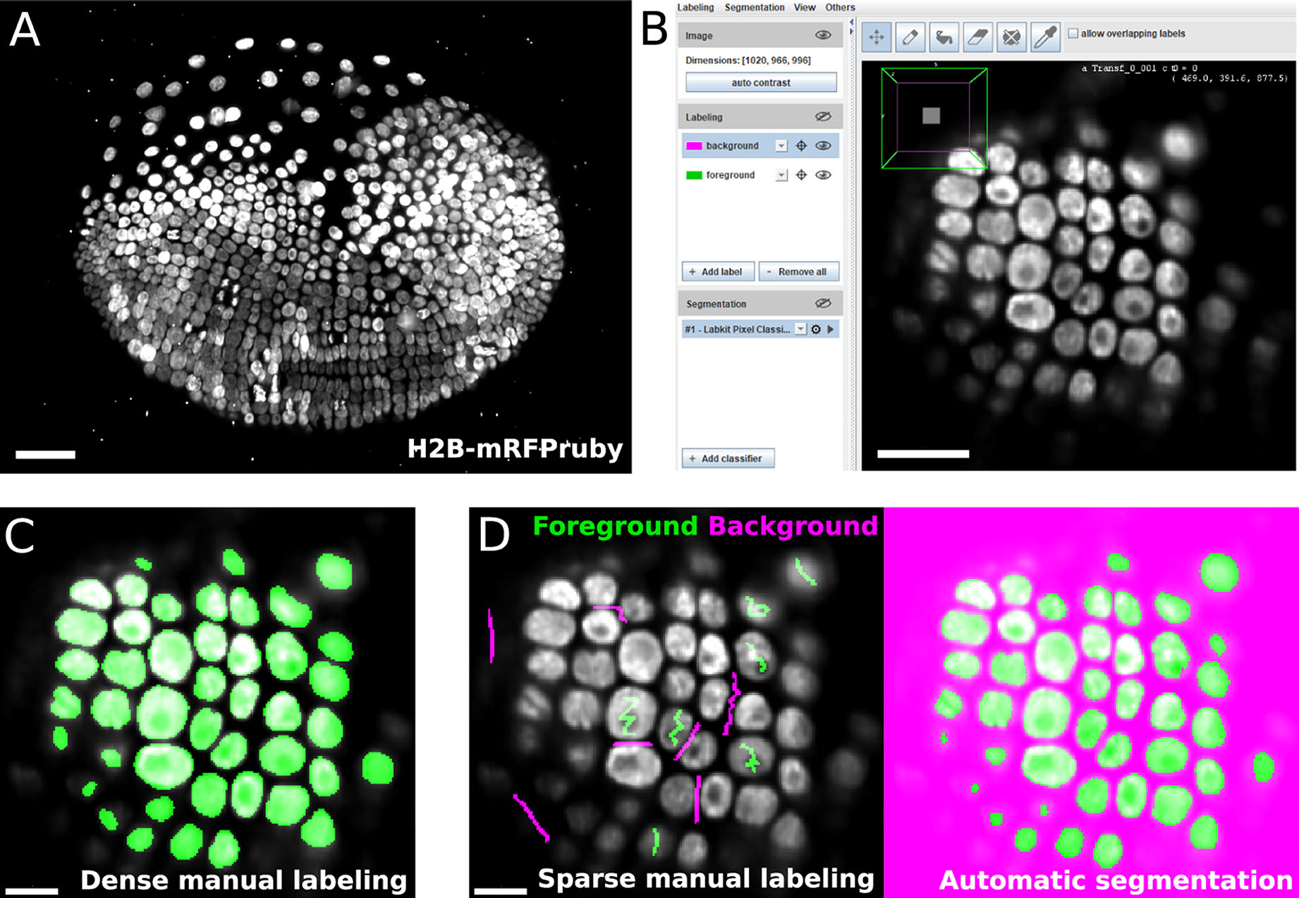
Figure 1. LABKIT allows easy manual labeling and automatic segmentation of large image volumes: (A) Maximum intensity projection of a single time point from a ~1 TB timelapse of a developing Parhyale embryo imaged live with lightsheet microscopy. (B) LABKIT's user interface is based on BigDataViewer and allows visualizing and interacting with large volumes of image data. A slice of the developing Parhyale embryo is shown. (C) Users can label large datasets with dense manual annotations using LABKIT's drawing interface. (D) A core feature of LABKIT is the rapid segmentation of large image data using sparse manual labels (scribbles) combined with random forest pixel classification to automatically produce the final segmentation. Scale bars 100 μm (A), 50 μm (B), and 25 μm (C,D).

Thanks to the intuitive interface design, users can efficiently segment their images by manually drawing dense labels on the entire image (Figure 1C). Labels that are generated with the drawing tools can directly be saved as images or exported to Fiji for downstream processing. Dense manual labelings of complete images or volumes created with LABKIT can be used to manually segment objects, as was done previously to mask particles in cryo-electron tomograms of Chlamydomonas (Jordan and Pigino, 2019).

However, this process is very time consuming and doesn't scale well to large data. LABKIT is therefore often used to densely and manually label a subset of the image data, which is then used as ground-truth for supervised deep learning approaches. Published examples include the generation of ground-truth training data for a mouse and a Platyneris dataset in order to segment cell nuclei with EmbedSeg (Lalit et al., 2021). LABKIT is also suggested as a tool of choice for ground-truth generation by other deep learning methods (Schmidt et al., 2018; Buchholz et al., 2020; Horlava et al., 2020). Still, manually generating sufficient amount of ground-truth training labels for existing deep learning methods remains a cumbersome and tedious task.

In order to create a high quality segmentation while maintaining low user input, LABKIT features a random forest (Breiman, 2001) based pixel classification algorithm, with all feature computations optimized for quick runtimes. Instead of annotating entire objects, a random forest is trained on a few pixel labeling per class only. These sparse manual labels, or scribbles (see Figure 1D, left), are directly drawn by users over the image. Naturally, scribbles must be drawn on pixels representative of each class. Once trained, the random forest classifier enables the generation of a segmentation (dense pixel classification, see Figure 1D). Two or more classes can be used to distinguish foreground objects from background pixels. Figures 2A,B showcase examples of a single foreground and background classes. If desired, out of focus objects can even be discarded, for example by making such pixels part of the background class (Figure 2B, arrowheads). For more complex segmentation tasks that need to discriminate various visible structures (e.g., nucleus vs. cytoplasm vs. background) or cell types (as in Figure 2C), two or more foreground classes can be used (Figure 2D).

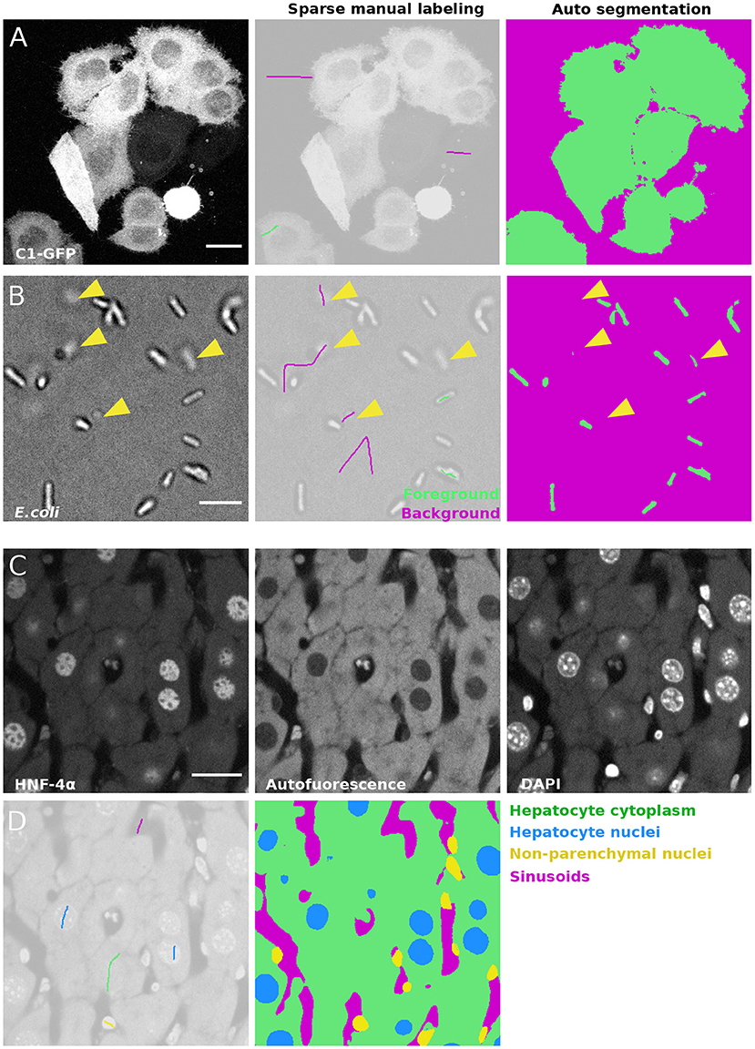
Figure 2. Semantic segmentation of microscopy images with LABKIT's pixel classification: (A) Maximum intensity projection of a confocal stack showing HeLa cells expressing C1-GFP (left), next to the sparse labeling (scribbles, center) and resulting cell segmentation (right). (B) Bright field microscopy image of E.coli, sparse labeling discriminating cells and background and the resulting segmentation. Arrowheads show that segmentation of out-of-focus objects can be reduced by including pixels of such objects in the background class. (C) Fixed mouse liver tissue section stained with immunofluorescence and imaged in multiple channels with a spinning disk confocal microscope, showing Hepatocyte nuclei stained with antibody against HNF-4α a transcription factor expressed in hepatocytes, hepatocyte cytoplasm (autofluorescence) and all nuclei stained with DAPI. (D) Labeling and resulting segmentation of the liver tissue section shown in (A), segmenting Hepatocyte cytoplasm (green), Hepatocyte nuclei (blue), nuclei of non-parenchymal cells (yellow) and sinusoids (magenta). Scale bars 20 μm (A), (C), and 5 μm (B).

As opposed to deep learning algorithms, random forests are typically trained in a matter of seconds. Drawing scribbles and computing the segmentation can therefore conveniently be iterated due to the efficient parallelization we have implemented, leading to live segmentation. Live results are computed and displayed only on the currently visualized image slice in BigDataViewer to increase the interactivity. Hence, the effect of additional scribbles (sparse labels) is instantly visible and users can stop once the automated output of the pixel classifier reaches sufficient quality. This iterative workflow makes working with LABKIT very efficient, even when truly large image data are being processed. BigDataViewer's bookmarking feature can additionally be used to quickly jump between previously defined image regions, thereby allowing validating the quality of the pixel classifier on multiple areas. Since we use ImgLib's caching infrastructure, all image blocks that have once been computed are kept in memory and switching between bookmarks or browsing between parts of a huge volume is fast and visually pleasing. Once sufficiently trained, the classifier can be saved for later use in interactive LABKIT sessions or in Fiji/ImageJ macros. The entire dataset can be directly segmented and the results saved to disk. Recently, sparse labeling combined with random forest pixel classification in LABKIT was used to segment mice epidermal cells (Bornes et al., 2021), as well as mRNA foci in neurons (Arshadi et al., 2021).

Once the image is fully segmented, the generated segmentation masks can be transferred to label layers and the drawing tools can now be used to curate them. The goal of curation is to resolve the remaining errors made by the trained pixel classifier, such as drawing missing parts, filling holes, erasing mislabeling and deleting spurious blobs (Figure 3). Label curation is performed until the curated segmentation is deemed satisfactory for downstream processing or analysis. LABKIT can also be used to curate segmentation results obtained by other methods that are not available within LABKIT, including deep learning based methods (Jain et al., 2020).

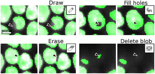
Figure 3. LABKIT labeling tools used for curation: labels generated by manual dense labeling or automatic segmentation can be efficiently curated with drawing, filling, erasing, or deletion of entire objects. Scale bar 10 μm.

Automated segmentation with LABKIT and the possibility to quickly curate any automated segmentation result make LABKIT a powerful tool that can considerably shorten the time required to generate ground-truth data for training deep learning approaches. For example, we compared automatic and manual segmentation with LABKIT on a rather small subset of images (N=26, see one example in Figure 4A) made publicly available by the 218 Data Science Bowl (Caicedo et al., 2019). We segmented all images within 5 min by iterative scribbling and automated segmentation (see Figure 4B). While many images consisted of homogeneous nuclei and led to high quality results, images with heterogeneous nuclei resulted in segmentation errors (see arrows in Figure 4B). Such errors include spurious instances that do not correlate with any object in the original image, instances that correspond to the fusion of multiple instances, instances with holes, or even instances that split in two. Such errors are obviously undesirable and negatively impact the overall average precision score (AP = 0.72, see Methods for the metrics definition). As described above, all such segmentation errors can easily be corrected within LABKIT, either by adding sparse labels corresponding to typical areas with errors, done during the iterative process, or when they persist by manually curating the residual errors in the final automated results (Figure 4C). Curating all 26 images took an additional 10 min and raised the corresponding average precision to 0.76, a score very close to the inter-observer distance (AP = 0.78), as shown in Figures 4C,D. In contrast, manually segmenting all images required more than an hour (Figure 4D), which is four times longer than scribble-based pixel classification with LABKIT, followed by full curation of the results to obtain images of comparable quality.

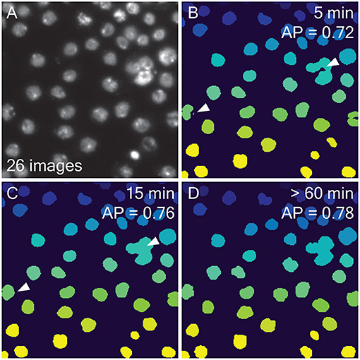
Figure 4. Comparing automatic and manual ground-truth generation with LABKIT: (A) Fluorescence image of nuclei (out of 26 images) extracted from the 2018 Data Science Bowl (Caicedo et al., 2019). (B) Results from LABKIT automated segmentation of (A) after extracting connected components and giving each instance a unique pixel value. The arrows point to various segmentation errors. On the top right corner, the total time necessary to obtain the corresponding segmentation of all 26 images (including labeling) is indicated. Below the timing is the average precision (see Methods) as compared to a dense manual labeling performed by another observer. (C) Curation of (B) with same post-processing. The arrows point to the corrected errors mentioned in (B). The timing information includes (B). (D) Dense manual labeling of (A) and the same post-processing as in (B). No scale bar was available for the images.

Hence, whenever LABKIT automated segmentation is by itself not sufficient, manually curating the results yields ground-truth data that can be used to train a deep learning method, leading to higher segmentation quality with less labeling effort.

3. LABKIT Pixel Classifier

LABKIT provides a pixel classification algorithm for automatic segmentation. The algorithm uses a random forest to classify each pixel independently into user-defined classes (e.g., foreground and background). Random Forests (Breiman, 2001) are widely used supervised machine learning methods, and as such must be trained on a given body of ground-truth labels (pre-classified example pixels). In LABKIT, the random forest classifier is trained on manually labeled pixels (scribbles), an approach similar to ilastik (Berg et al., 2019) or Trainable Weka Segmentation (Arganda-Carreras et al., 2017). As opposed to most implementations, LABKIT's classifier is specifically optimized to be able to handle very large image data.

In a first step, we compute a feature vector for each labeled pixel. This is achieved by applying a configurable set of filters to the given image or images. To this end LABKIT offers a set of image filters commonly used in image analysis, such as Gaussian, difference of Gaussians or Laplacian filters. Each selected filter creates an output image that emphasizes different features of a given input image. Filter responses for each pixel are then added to their feature vector. The final feature vectors of all labeled pixels are paired with their respective ground-truth classes, together constituting the training set. This data is then used to train the random forest, consisting of 100 decision trees, using the FastRF library (Supek, 2015).

After training, the random forest classifier can predict pixel classes directly from the feature vector of any given pixel. Hence, in a final step, we apply the random forest to the feature vectors of all pixels in the entire body of data, thereby effectively computing the desired semantic segmentation.

Since computing feature vectors and final random forest predictions consume by far the most computational resources, it was crucial to optimize their runtime. To this end, we process image chunks in parallel, with the chunked memory handling being supported by ImgLib2 (Pietzsch et al., 2012). Additionally, we implemented OpenCL kernels, allowing us to benefit from fast GPU computations (Haase et al., 2020).

4. Limitations of the Pixel Classification

The simplicity of the pixel classification algorithm ensures efficiency, but also exposes it to certain limitations and potential failure modes. This mainly comes from the fact that the filter kernels used to compute the feature vector have limited sizes. With the default settings in LABKIT, filters respond mostly to a 16x16 window (2D), meaning that decision about the class of a given pixel is based on filter responses in a small neighborhood. A direct consequence is illustrated in Figure 5A, where LABKIT was used to segment the image of a vacuole pore in paramecium caudatum (left panel) using three classes: inner pore (central panel, in blue), vacuole (in green) and background (in magenta). Because inner pore and background pixels have similar texture, the classifier cannot tell them apart and assigns background pixels to the inner pore class, and vice versa.

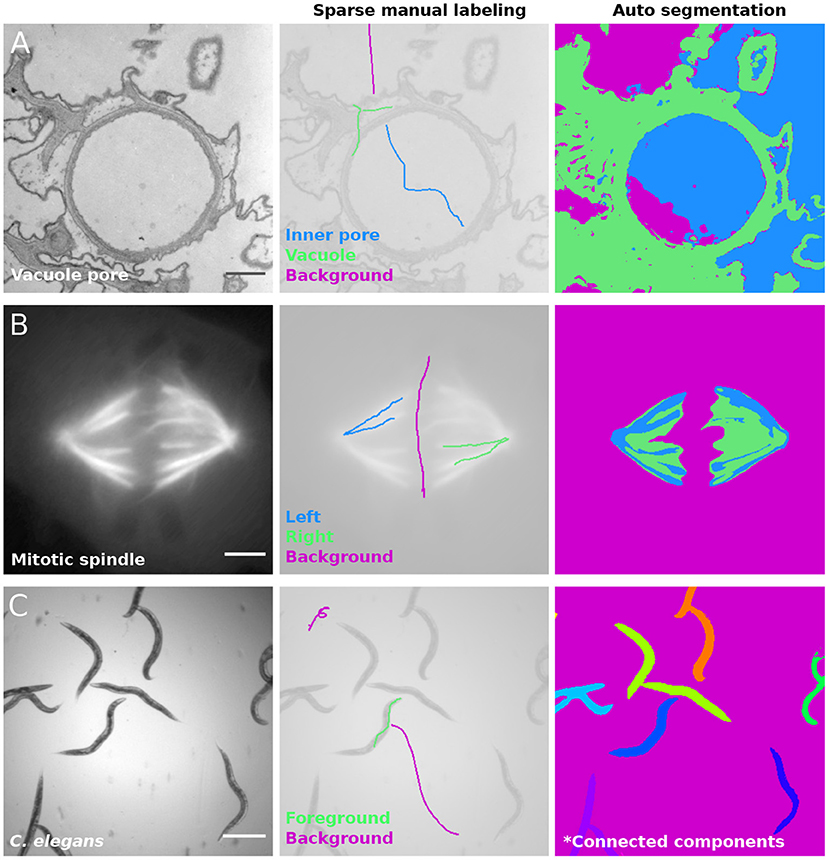
Figure 5. Pixel classification failure modes: (A) Image of a contractile vacuole pore in paramecium caudatum acquired with transmission electron microscopy (left), in which inner pore (blue), cytoplasm (green) and background (magenta) were labeled with scribbles (center). LABKIT's classifier fails to distinguish background and inner pore classes (right). Image provided by Richard Allen (Cell Image Library, 38894). (B) Mitotic spindle of a Ptk2 cell expressing GFP-tubulin imaged in wide-field fluorescence (left). Left and right halves of the mitotic spindle are labeled in different classes (blue and green, respectively), while background is labeled in magenta (center). LABKIT's classifier is incapable of discriminating similar structures (right). Image provided by Sophie Dumont and Timothy J. Mitchison (Cell Image Library, 6568). (C) Bright field image of C. elegans (left), labeled with two classes (center): foreground (green) and background (magenta). After applying connected components analysis to the classification result, contiguous worms belong to the same object (right). Image provided by Fred Ausubel (Broad Bioimage Benchmark Collection, BBBC010). Scale bars (A) 500 nm, (B) 10 μm, and (C) 500 μm.

All filters used to calculate the feature vectors are designed to be translation and rotation invariant. Hence, the algorithm classifies two objects the same way regardless of their position or orientation in the image. While this is a sensible assumption for most applications on microscopy data, users should certainly be aware of this. One potential problem is showcased in Figure 5B, which shows a mitotic spindle in fluorescence microscopy (left) and an attempt at assigning each half of the mitotic spindle to a different class (central panel). Although both sides of the mitotic spindle are spatially distinct and in different orientations, the classifier fails at discriminating them (Figure 5B, right).

Furthermore, contiguous objects cannot be separated by the random forest classifier. This is illustrated in Figure 5C, which shows C. elegans worms imaged in bright-field microscopy (left panel). While the classifier can correctly distinguish the worms body from the background, a connected component analysis applied to the classification result (Figure 5C, right) leads to multiple worms being fused within the same connected component. In order to obtain instance segmentation from such images, manual curation or post-processing, such as watershed, is necessary to separate the connected objects into different instances.

Finally it is also important to know that trained random forest classifier cannot easily be trained on sets of very diverse images. Deep learning approaches such as Cellpose (Stringer et al., 2021), in contrast, show much greater potential to generalize well even when trained on a large and diverse body of microscopy data.

Nonetheless, LABKIT can be used to segment a wide range of images fast and at high quality. This is true as long as objects are visibly separated from one another and can be distinguished by the filter responses LABKIT computes per pixel.

5. Software and Workflow Integration

LABKIT's automatic segmentation is not limited to the dataset it was trained on. Because the trained classifier can be saved for later use, it can be applied to similar new images. While ensuring reproducibility of the results, it also helps maintaining consistency in the image segmentation. Manually loading both images and trained classifier in LABKIT for multiple sets of images is a repetitive task ill-suited for an automated workflow. Therefore, to simplify the integration into existing workflows in Fiji, LABKIT can be easily called from the ImageJ macro language. For instance, a simple macro script can open multiple datasets and segment each of them using a trained classifier.

Image segmentation can be further accelerated by running the process on GPUs thanks to CLIJ (Haase et al., 2020). Once CLIJ is properly set up, GPU acceleration is available for LABKIT in both graphical interface and macro commands. GPU processing is particularly beneficial in the case of large images, for which it allows shortening the lengthy segmentation tasks. Performing GPU-accelerated segmentation in LABKIT is a matter of activating a checkbox, and does not present additional complexity to users.

Some images, however, are far too large to be processed on a consumer machine in a reasonable amount of time, if they can be stored at all on such a computer. For such data, modern workflows resort to the use of HPC clusters, which are purposely built for high computing performances with large available memory. LABKIT offers a command line tool (Arzt, 2021a) allowing advanced users to segment images on HPC clusters.

The capability of extending LABKIT and re-using its components is illustrated by integration with the commercial Imaris software (Oxford Instruments, UK) via the recently released ImgLib2-Imaris compatibility bridge. In this context, LABKIT operates directly on datasets that are transparently shared (without duplication) between Imaris and ImgLib2 (Pietzsch et al., 2012). These datasets can be arbitrarily large, as both Imaris and ImgLib2 implement sophisticated caching schemes. In the same fashion, output segmentation masks are transparently shared with the running Imaris application, making additional file import/export steps unnecessary. Importantly, this functionality can also be triggered and controlled directly from Imaris to integrate it into streamlined object segmentation workflows.

6. Performance of LABKIT

In order to process large images on consumer computers, software packages must be able to load the data in memory, process it and save the results, all within the constraints of the machine. In LABKIT, this is achieved by reading only the portions of the image that are displayed to the user, thanks to the use of the HDF5 format (Folk et al., 2011) and the BigDataViewer (Pietzsch et al., 2015). The image is further processed in chunks using ImgLib2 (Pietzsch et al., 2012). As a result, LABKIT is capable of processing arbitrarily large images and is compatible with GPU acceleration and distributed computation on HPC clusters.

To illustrate this, we segmented a 13.4 gigapixel image (482 x 935 x 495 x 60 pixels, 25 GB) on a single laptop computer, with and without GPU, and with different nodes of an HPC cluster (see Table 1). The image was extracted and 2x down-sampled from the Fluo-N3DL-TRIF dataset made available for the Cell Tracking Challenge (Maška et al., 2014; Ulman et al., 2017; Jain et al., 2020) benchmark competition. Running the segmentation on the laptop using GPU acceleration sped up the computation by 7.5 fold, illustrating the benefit of harnessing GPU power for processing large images. While running computation on an HPC cluster comes with overhead, increasing the number of CPU nodes shortens the computation dramatically, reaching a 40-fold improvement from 1 CPU node to 50. Finally, GPU nodes on an HPC allow for more parallelization of the computation and therefore even higher computational speed-up on the segmentation task, with 10 GPU nodes processing the data in slightly over a minute.

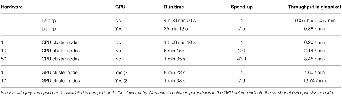
Table 1. Benchmarking computation speed while segmenting a large biological image on various hardware: the experiment was performed on a laptop with and without GPU acceleration, and on different numbers of CPU and GPU cluster nodes.

Furthermore, we trained and optimized a classifier on the Fluo-N3DL-TRIF dataset (original sampling), the largest dataset of the Cell Tracking Challenge (training dataset of size 320 GB, evaluation dataset of size 467 GB), and submitted it for evaluation against undisclosed ground-truth. The segmentation of both training and evaluation datasets was performed on an HPC cluster. LABKIT pixel classification ranked as the highest performing segmentation method on this dataset for all three evaluation metrics (OP_CSB, SEG and DET) (CTC, 2021). More specifically, LABKIT segmentation obtained the following scores: OP_CSB = 0.895 (0.886 for the second highest scoring entry), SEG = 0.793 (0.776) and DET = 0.997 (0.997), performing better than the other entries, including classical (bandpass segmentation) or deep learning (convolution neural network) algorithms. As opposed to the deep learning algorithm to which it was compared, Labkit only used a few hundred pixels as ground-truth, distributed throughout a small fraction of the training dataset (7 frames). Finally, LABKIT's classifier was simply trained through the LABKIT graphical interface, illustrating its ease of use.

7. Discussion and Conclusion

LABKIT is a labeling software tool designed to be intuitive and simple to use. It features a robust pixel classification algorithm aimed at segmenting images between multiple classes with very little manual labeling required. Similar to other tools of the BigDataViewer family (Pietzsch et al., 2015; Wolff et al., 2018; Hörl et al., 2019; Tischer et al., 2020), it integrates seamlessly into the SciJava and Fiji ecosystem. It can be easily installed through Fiji and incorporated into established workflows using ImageJ's macro language. The results of LABKIT's segmentation can be further analyzed in Fiji or exported to other software platforms, such as CellProfiler (McQuin et al., 2018), QuPath (Bankhead et al., 2017), or Ilastik (Berg et al., 2019).

Manual labeling, in both 2D and 3D, is also made easy by LABKIT. Other alternatives exist, among which QuPath (Bankhead et al., 2017) (2D), napari (napari contributors, 2019) or Paintera (Leite et al., 2021). In particular, Paintera is specifically tailored to 3D labeling of crowded environment, but at the cost of a steeper learning curve.

LABKIT is compatible with a wide range of image formats since image data can be loaded directly from Fiji using Bio-Formats (Linkert et al., 2010). Nonetheless, in order to fully benefit from LABKIT optimizations for large images, users must first convert their terabyte-sized images to a file format allowing high-speed access to arbitrary located sub-regions of the image. This strategy is also employed by other software, with the example of Ilastik (Berg et al., 2019). One such format is HDF5 (Folk et al., 2011), and LABKIT uses in particular the BigDataViewer HDF5+XML variant. In Fiji, images can easily be saved in this format using BigStitcher (Hörl et al., 2019) or Multiview-Reconstruction (Preibisch et al., 2014; Icha et al., 2016).

In the Cell Tracking Challenge (Ulman et al., 2017; CTC, 2021), LABKIT segmentation outperformed other entries on a particular dataset, one being a deep learning approach. This method was designed as part of a cell segmentation and tracking pipeline on various images, and it is likely that recent and specialized deep learning segmentation algorithms, such as StarDist (Schmidt et al., 2018) or CellPose (Stringer et al., 2021), would perform overall better (Baltissen et al., 2018; Morone et al., 2020). Yet, the full potential of deep learning algorithms is only reached when a sufficient amount of ground-truth data is available, which is too frequently the limiting factor. Generating ground-truth data for a deep learning method is a tedious endeavor without the insurance of a perfect segmentation result. A safer strategy is therefore to first try shallow learning for segmentation tasks, before even thinking of moving to deep learning algorithms. In cases where higher segmentation quality is truly necessary, curated results from shallow learning can be used to generate the massive amount of ground-truth required to train a deep learning algorithm. As seen previously, LABKIT is useful in all these scenarios since it can be used to manually generate ground-truth annotations or to segment the images with shallow learning before curating the results in order to use them as ground-truth for other learning-based algorithms (see Figure 6).

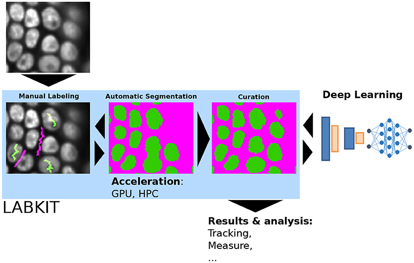
Figure 6. LABKIT's iterative and interactive segmentation used for ground-truth generation: manual labeling, automatic segmentation and curation in LABKIT enable easy and rapid image segmentation, whose results can be further processed or used as ground-truth for deep-learning classifiers.

In the future, we intend to extend LABKIT's functionalities to improve manual and automated segmentation. For instance, we will add a magic wand tool to select, fill, fuse or delete labels based on the pixel classification. Furthermore, we aim to add new segmentation algorithms, such as the deep learning algorithm DenoiSeg (Buchholz et al., 2020) already available in Fiji. In recent years, novel interactive deep learning approaches have also been shown to reduce the need for large amounts of densely labeled ground-truth data. In general, these approaches combine deep learning with interactive user guidance, for instance clicks on the extreme points of objects (Maninis et al., 2018), inside-outside guidance (Zhang et al., 2020), clicks within objects and boundaries that are iteratively refined (Luo et al., 2021) and a combination of clicks and squiggles inside objects (Alemi Koohbanani et al., 2020). However, these approaches are not in widespread use in bio-image analysis and for the most part implemented in Python. LABKIT could potentially serve as an easy-to-use platform for such methods by implementing their labeling strategies in the user interface and interfacing their framework with Java, thereby making them widely accessible to the biomedical community. LABKIT source code is open source and can be found online (Arzt, 2021b), together with its command-line interface (Arzt, 2021a), tutorials and documentation (Arzt, 2021c).

8. Methods

8.1. Timing Instance Segmentation Generation

The dataset consisted of all 256 x 256 images (N = 26) in the test sample of StarDist (Schmidt et al., 2018), originally published as part of the 2018 Data Science Bowl (Caicedo et al., 2019) (subset of stage1_train, accession number BBBC038, Broad Bioimage Benchmark Collection). The images were loaded in LABKIT as a stack and sparsely labeled (scribbles). A classifier was then trained with the default filter settings: “original image,” “Gaussian blur,” “difference of Gaussians,” “Gaussian gradient magnitude,” “Laplacian of Gaussian,” and “Hessian eigenvalues,” with sigma values: 1, 2, 4, and 8. The results were saved and then manually curated using the brush and eraser tools. Finally, the same original image stack was densely manually labeled afresh. The total time required to process all images was measured using a chronometer for i) LABKIT automated segmentation, including the sparse manual labeling, ii) the previous step followed by a curation step and iii) dense manual labeling. In order to evaluate the segmented images, connected components were computed (4-connectivity) and given unique pixel values (instance segmentation). Quality metrics scores were calculated as the average precision with threshold 0.5 as defined in StarDist (Schmidt et al., 2018). We used dense manual labeling performed by another observer as reference images, and computed the metrics score for the results obtained in i), ii), and iii). The average metrics over the images were calculated as a weighted average of each individual image, where the weights were the number of instances in the reference image.

8.2. Speed Benchmark

The dataset was downloaded from the Cell Tracking Challenge (Ulman et al., 2017) website, and consisted of the first training dataset of the Fluo-N3DL-TRIF example. The dataset was down-sampled by a factor 2 in order to reduce its size and simplify the benchmarking. The dataset was then saved in the BigDataViewer XML+HDF5 format using BigStitcher (Hörl et al., 2019). LABKIT was used to draw a few scribbles on both background and nuclei areas, and to train a random forest classifier using the default settings. The trained model was then saved. The LABKIT command line tool was used to run the benchmark experiment on a Dell XPS 15 laptop (32 MB RAM, Intel Core i7-6700HQ CPU with 8 cores, GeForce GTX 960M GPU) and on an HPC cluster, with both CPU (256 GB RAM, Intel Xeon CPU E5-2680 v3 with 2.5 GHz and 24 cores) and GPU (512 GB RAM, Intel Xeon CPU E5-2698 v4 with 2.2 GHz and 40 cores, with two GeForce GTX 1080 GPUs) nodes. The segmentation results on the HPC were saved in the N5 (Saalfeld, 2017) format to maximize writing speed. Benchmarking included read/write of image data form disc, optional data transfer to the GPU, computation of feature images and classification all together.

8.3. Cell Tracking Challenge

As in the speed benchmark sample, all Fluo-N3DL-TRIF datasets (training and evaluation) were converted to BigDataViewer XML+HDF5 format using the BigStitcher Fiji plugin. This time, however, no down-sampling was applied to the images. For training, only frames 0, 1, 10, 20, 40, 50 and 59 from sequence “01” of the training dataset were used. A few hundred pixels were labeled as foreground and background. Only nuclei's central pixels were labeled as foreground in order to force the classification algorithm to return segments of smaller size than the actual nuclei. Thus, segmented nuclei are unlikely to touch and segmentation errors are minimized. We used the following filters to train the random forest classifier: “original image,” “Gaussian blur,” “Laplacian of Gaussian,” and “Hessian eigenvalues,” with sigma values 1, 2, 4, 8, and 16. The filters can be set in LABKIT's interface through the parameters menu of the classifier. The trained classifier was saved and the evaluation dataset was segmented using the LABKIT command line tool on an HPC. Since the output of the pixel classification is a binary mask, we performed a connected component analysis to assign unique pixel values to the individual segments. Finally, we dilated the segments to match the size of the nuclei. The dilation was done in three steps: the first two steps with a three-dimensional 6-neighborhood dilation kernel, then with a 3 x 3 x 3 pixel cube kernel. The combination of dilation kernels was chosen as to optimize the SEG score on the training dataset. All metrics scores were computed by the Cell Tracking Challenge platform.

Data Availability Statement

Publicly available datasets were analyzed in this study. This data can be found here: http://cellimagelibrary.org/images/38894, accession number CIL:38894, Cell Image Library, http://cellimagelibrary.org/images/6568, accession number CIL:6568, Cell Image Library, https://bbbc.broadinstitute.org/BBBC010, accession number BBBC010, Broad Bioimage Benchmark Collection, https://bbbc.broadinstitute.org/BBBC038, accession number BBBC038, Broad Bioimage Benchmark Collection and http://celltrackingchallenge.net/3d-datasets/, Fluo-N3DL-TRIF dataset, Cell Tracking Challenge.

Author Contributions

FJ, MA, TP, PT, and DS designed the project. MA implemented the software with help from TP, DS, and RH. MA and JD performed experiments. MA, JD, CS, and FJ wrote the manuscript with inputs from all authors.

Funding

Funding was provided from the Max-Planck Society under project code M.IF.A.MOZG8106, the core budget of the Max-Planck Institute of Molecular Cell Biology and Genetics (MPI-CBG), the Human Technopole, and the BMBF under codes 031L0102 (de.NBI) and 01IS18026C (ScaDS2), as well as by the Deutsche Forschungsgemeinschaft (DFG) under code JU3110/1-1 (FiSS) and TO563/8-1 (FiSS). PT was supported by the European Regional Development Fund in the IT4Innovations national supercomputing center, project number CZ.02.1.01/0.0/0.0/16_013/0001791 within the Program Research, Development and Education. RH acknowledges support by the DFG under Germany's Excellence Strategy–EXC2068-Cluster of Excellence Physics of Life of TU Dresden.

Conflict of Interest

The authors declare that the research was conducted in the absence of any commercial or financial relationships that could be construed as a potential conflict of interest.

Publisher's Note

All claims expressed in this article are solely those of the authors and do not necessarily represent those of their affiliated organizations, or those of the publisher, the editors and the reviewers. Any product that may be evaluated in this article, or claim that may be made by its manufacturer, is not guaranteed or endorsed by the publisher.

Acknowledgments

We thank Anne Wuttke (Zerial lab, MPI-CBG), Sascha Kuhn (Nadler lab, MPI-CBG), Maria Luisa Romero Romero (Toth-Petroczy lab, MPI-CBG), Akanksha Jain & Anastasios (Tassos) Pavlopoulos (Tomancak, MPI-CBG) for sharing the experimental data. We also want to thank the Scientific Computing Facility at MPI-CBG for giving us access to HPC infrastructure.

References

Alemi Koohbanani, N., Jahanifar, M., Zamani Tajadin, N., and Rajpoot, N. (2020). Nuclick: a deep learning framework for interactive segmentation of microscopic images. Med. Image Anal. 65:101771. doi: 10.1016/j.media.2020.101771
Arganda-Carreras, I., Kaynig, V., Rueden, C., Eliceiri, K. W., Schindelin, J., Cardona, A., et al. (2017). Trainable weka segmentation: a machine learning tool for microscopy pixel classification. Bioinformatics 33, 2424–2426. doi: 10.1093/bioinformatics/btx180
Arshadi, C., Günther, U., Eddison, M., Harrington, K. I. S., and Ferreira, T. A. (2021). SNT: a unifying toolbox for quantification of neuronal anatomy. Nat. Methods 18, 374–377. doi: 10.1038/s41592-021-01105-7
Arzt, M. (2021a). Available online at: https://github.com/juglab/labkit-command-line (accessed December 09, 2021).
Arzt, M. (2021b). Available online at: https://github.com/juglab/labkit-ui (accessed December 09, 2021).
Arzt, M. (2021c). Available online at: https://imagej.net/plugins/labkit (accessed December 09, 2021).
Baltissen, D., Wollmann, T., Gunkel, M., Chung, I., Erfle, H., Rippe, K., et al. (2018). “Comparison of segmentation methods for tissue microscopy images of glioblastoma cells,” in 2018 IEEE 15th International Symposium on Biomedical Imaging (ISBI 2018) (Washington, DC: IEEE), 396–399.
Bankhead, P., Loughrey, M. B., Fernández, J. A., Dombrowski, Y., McArt, D. G., Dunne, P. D., et al. (2017). Qupath: Open source software for digital pathology image analysis. Sci. Rep. 7, 1–7. doi: 10.1038/s41598-017-17204-5
Berg, S., Kutra, D., Kroeger, T., Straehle, C. N., Kausler, B. X., Haubold, C., et al. (2019). Ilastik: interactive machine learning for (bio) image analysis. Nat. Methods 16, 1226–1232. doi: 10.1038/s41592-019-0582-9
Betzig, E., Patterson, G. H., Sougrat, R., Lindwasser, O. W., Olenych, S., Bonifacino, J. S., et al. (2006). Imaging intracellular fluorescent proteins at nanometer resolution. Science 313, 1642–1645. doi: 10.1126/science.1127344
Bornes, L., Windoffer, R., Leube, R. E., Morgner, J., and van Rheenen, J. (2021). Scratch-induced partial skin wounds re-epithelialize by sheets of independently migrating keratinocytes. Life Sci. Alliance 4, e202000765. doi: 10.26508/lsa.202000765
Buchholz, T.-O., Prakash, M., Krull, A., and Jug, F. (2020). DenoiSeg: joint denoising and segmentation. arXiv:2005.02987 [cs]. arXiv: 2005.02987. doi: 10.1007/978-3-030-66415-2_21
Caicedo, J. C., Goodman, A., Karhohs, K. W., Cimini, B. A., Ackerman, J., Haghighi, M., et al. (2019). Nucleus segmentation across imaging experiments: the 2018 data science bowl. Nat. Methods 16, 1247–1253. doi: 10.1038/s41592-019-0612-7
CTC (2021). Available online at: http://celltrackingchallenge.net/latest-csb-results (accessed December 09, 2021).
Denk, W., and Horstmann, H. (2004). Serial block-face scanning electron microscopy to reconstruct three-dimensional tissue nanostructure. PLoS Biol. 2:e329. doi: 10.1371/journal.pbio.0020329
Dodt, H.-U., Leischner, U., Schierloh, A., Jährling, N., Mauch, C. P., Deininger, K., et al. (2007). Ultramicroscopy: three-dimensional visualization of neuronal networks in the whole mouse brain. Nat. Methods 4, 331–336. doi: 10.1038/nmeth1036
Folk, M., Heber, G., Koziol, Q., Pourmal, E., and Robinson, D. (2011). “An overview of the hdf5 technology suite and its applications,” in Proceedings of the EDBT/ICDT 2011 Workshop on Array Databases (Uppsala), 36–47.
Gustafsson, M. G. (2000). Surpassing the lateral resolution limit by a factor of two using structured illumination microscopy. J. Microsc. 198, 82–87. doi: 10.1046/j.1365-2818.2000.00710.x
Haase, R., Royer, L. A., Steinbach, P., Schmidt, D., Dibrov, A., Schmidt, U., et al. (2020). Clij: Gpu-accelerated image processing for everyone. Nat. Methods 17, 5–6. doi: 10.1038/s41592-019-0650-1
Hama, H., Kurokawa, H., Kawano, H., Ando, R., Shimogori, T., Noda, H., et al. (2011). Scale: a chemical approach for fluorescence imaging and reconstruction of transparent mouse brain. Nat. Neurosci. 14, 1481–1488. doi: 10.1038/nn.2928
Hell, S. W., and Wichmann, J. (1994). Breaking the diffraction resolution limit by stimulated emission: stimulated-emission-depletion fluorescence microscopy. Opt. Lett. 19, 780–782. doi: 10.1364/OL.19.000780
Hess, S. T., Girirajan, T. P., and Mason, M. D. (2006). Ultra-high resolution imaging by fluorescence photoactivation localization microscopy. Biophys. J. 91, 4258–4272. doi: 10.1529/biophysj.106.091116
Hörl, D., Rusak, F. R., Preusser, F., Tillberg, P., Randel, N., Chhetri, R. K., et al. (2019). Bigstitcher: reconstructing high-resolution image datasets of cleared and expanded samples. Nat. Methods 16, 870–874. doi: 10.1038/s41592-019-0501-0
Horlava, N., Mironenko, A., Niehaus, S., Wagner, S., Roeder, I., and Scherf, N. (2020). A comparative study of semi- and self-supervised semantic segmentation of biomedical microscopy data. arXiv:2011.08076 [cs, stat]. arXiv: 2011.08076.
Huisken, J., Swoger, J., Del Bene, F., Wittbrodt, J., and Stelzer, E. H. (2004). Optical sectioning deep inside live embryos by selective plane illumination microscopy. Science 305, 1007–1009. doi: 10.1126/science.1100035
Icha, J., Schmied, C., Sidhaye, J., Tomancak, P., Preibisch, S., and Norden, C. (2016). Using light sheet fluorescence microscopy to image zebrafish eye development. J. Vis. Exp. 110:e53966. doi: 10.3791/53966
Jain, A., Ulman, V., Mukherjee, A., Prakash, M., Cuenca, M. B., Pimpale, L. G., et al. (2020). Regionalized tissue fluidization is required for epithelial gap closure during insect gastrulation. Nat. Commun. 11, 5604. doi: 10.1038/s41467-020-19356-x
Jordan, M. A., and Pigino, G. (2019). “Chapter 9-In situ cryo-electron tomography and subtomogram averaging of intraflagellar transport trains,” in Methods in Cell Biology, volume 152 of Three-Dimensional Electron Microscopy, eds T. Müller-Reichert and G. Pigino (Cambridge, MA: Academic Press), 179–195.
Knott, G., Marchman, H., Wall, D., and Lich, B. (2008). Serial section scanning electron microscopy of adult brain tissue using focused ion beam milling. J. Neurosci. 28, 2959–2964. doi: 10.1523/JNEUROSCI.3189-07.2008
Lalit, M., Tomancak, P., and Jug, F. (2021). Embedding-based Instance Segmentation in Microscopy. arXiv:2101.10033 [cs, eess]. arXiv: 2101.10033.
Leite, V., Saalfeld, S., Hanslovsky, P., Hulbert, C., Funke, J., Pietzsch, T., et al. (2021). Paintera. Zenodo. doi: 10.5281/zenodo.3351562
Linkert, M., Rueden, C. T., Allan, C., Burel, J.-M., Moore, W., Patterson, A., et al. (2010). Metadata matters: access to image data in the real world. J. Cell Biol. 189, 777–782. doi: 10.1083/jcb.201004104
Luo, X., Wang, G., Song, T., Zhang, J., Aertsen, M., Deprest, J., et al. (2021). Mideepseg: Minimally interactive segmentation of unseen objects from medical images using deep learning. Med. Image Anal. 72:102102. doi: 10.1016/j.media.2021.102102
Mais, L., Hirsch, P., and Kainmueller, D. (2020). “Patchperpix for instance segmentation,” in Computer Vision-ECCV 2020: 16th European Conference, Glasgow, UK, August 23–28, 2020, Proceedings, Part XXV 16 (Glasgow: Springer), 288–304.
Maninis, K.-K., Caelles, S., Pont-Tuset, J., and Van Gool, L. (2018). “Deep extreme cut: From extreme points to object segmentation,” in 2018 IEEE/CVF Conference on Computer Vision and Pattern Recognition (Salt Lake City: IEEE), 616–625.
Maška, M., Ulman, V., Svoboda, D., Matula, P., Matula, P., Ederra, C., et al. (2014). A benchmark for comparison of cell tracking algorithms. Bioinformatics 30, 1609–1617. doi: 10.1093/bioinformatics/btu080
McQuin, C., Goodman, A., Chernyshev, V., Kamentsky, L., Cimini, B. A., Karhohs, K. W., et al. (2018). Cellprofiler 3.0: Next-generation image processing for biology. PLoS Biol. 16:e2005970. doi: 10.1371/journal.pbio.2005970
Morone, D., Marazza, A., Bergmann, T. J., and Molinari, M. (2020). Deep learning approach for quantification of organelles and misfolded polypeptide delivery within degradative compartments. Mol. Biol.Cell. 31, 1512–1524. doi: 10.1091/mbc.E20-04-0269
Napari Contributors (2019). napari: A Multi-Dimensional Image Viewer For Python. Zenodo. doi: 10.5281/zenodo.3555620
Pietzsch, T., Preibisch, S., Tomančák, P., and Saalfeld, S. (2012). Imglib2–generic image processing in java. Bioinformatics 28, 3009–3011. doi: 10.1093/bioinformatics/bts543
Pietzsch, T., Saalfeld, S., Preibisch, S., and Tomancak, P. (2015). Bigdataviewer: visualization and processing for large image data sets. Nat. Methods 12, 481–483. doi: 10.1038/nmeth.3392
Preibisch, S., Amat, F., Stamataki, E., Sarov, M., Singer, R. H., Myers, E., et al. (2014). Efficient Bayesian-based multiview deconvolution. Nat. Methods 11, 645–648. doi: 10.1038/nmeth.2929
Rueden, C. T., Schindelin, J., Hiner, M. C., DeZonia, B. E., Walter, A. E., Arena, E. T., et al. (2017). Imagej2: imagej for the next generation of scientific image data. BMC Bioinformatics 18:529. doi: 10.1186/s12859-017-1934-z
Rust, M. J., Bates, M., and Zhuang, X. (2006). Sub-diffraction-limit imaging by stochastic optical reconstruction microscopy (storm). Nat. Methods 3, 793–796. doi: 10.1038/nmeth929
Saalfeld, S. (2017). Available online at: https://github.com/saalfeldlab/n5 (accessed December 17, 2021).
Schindelin, J., Arganda-Carreras, I., Frise, E., Kaynig, V., Longair, M., Pietzsch, T., et al. (2012). Fiji: an open-source platform for biological-image analysis. Nat Methods. 9, 676–682. doi: 10.1038/nmeth.2019
Schmidt, U., Weigert, M., Broaddus, C., and Myers, G. (2018). “Cell detection with star-convex polygons,” in International Conference on Medical Image Computing and Computer-Assisted Intervention (Berlin; Heidelberg: Springer), 265–273.
Schneider, C. A., Rasband, W. S., and Eliceiri, K. W. (2012). Nih image to imagej: 25 years of image analysis. Nat. Methods 9, 671–675. doi: 10.1038/nmeth.2089
Stringer, C., Wang, T., Michaelos, M., and Pachitariu, M. (2021). Cellpose: a generalist algorithm for cellular segmentation. Nat. Methods 18, 100–106. doi: 10.1038/s41592-020-01018-x
Supek, F. (2015). Available online at: https://code.google.com/archive/p/fast-random-forest/ (accessed December 09, 2021).
Tischer, C., Ravindran, A., Reither, S., Pepperkok, R., and Norlin, N. (2020). Bigdataprocessor2: a free and open-source fiji plugin for inspection and processing of tb sized image data. bioRxiv. doi: 10.1101/2020.09.23.244095
Ulman, V., Maška, M., Magnusson, K. E., Ronneberger, O., Haubold, C., Harder, N., et al. (2017). An objective comparison of cell-tracking algorithms. Nat. Methods 14, 1141–1152. doi: 10.1038/nmeth.4473
Wolff, C., Tinevez, J.-Y., Pietzsch, T., Stamataki, E., Harich, B., Guignard, L., et al. (2018). Multi-view light-sheet imaging and tracking with the mamut software reveals the cell lineage of a direct developing arthropod limb. Elif. 7:e34410. doi: 10.7554/eLife.34410
Wolny, A., Cerrone, L., Vijayan, A., Tofanelli, R., Barro, A. V., Louveaux, M., et al. (2020). Accurate and versatile 3d segmentation of plant tissues at cellular resolution. Elife 9:e57613. doi: 10.7554/eLife.57613
Keywords: segmentation, labeling, machine learning, random forest, Fiji, open-source
Citation: Arzt M, Deschamps J, Schmied C, Pietzsch T, Schmidt D, Tomancak P, Haase R and Jug F (2022) LABKIT: Labeling and Segmentation Toolkit for Big Image Data. Front. Comput. Sci. 4:777728. doi: 10.3389/fcomp.2022.777728
Received: 15 September 2021; Accepted: 13 January 2022;
Published: 10 February 2022.
Edited by:
Marcello Pelillo, Ca' Foscari University of Venice, ItalyReviewed by:
Xinggang Wang, Huazhong University of Science and Technology, ChinaCsaba Beleznai, Austrian Institute of Technology (AIT), Austria
Copyright © 2022 Arzt, Deschamps, Schmied, Pietzsch, Schmidt, Tomancak, Haase and Jug. This is an open-access article distributed under the terms of the Creative Commons Attribution License (CC BY). The use, distribution or reproduction in other forums is permitted, provided the original author(s) and the copyright owner(s) are credited and that the original publication in this journal is cited, in accordance with accepted academic practice. No use, distribution or reproduction is permitted which does not comply with these terms.
*Correspondence: Florian Jug, florian.jug@fht.org